Observatory#
The framework derives structures. This notebook plugs in measured values and asks: where do the observables sit?
import numpy as np
import matplotlib.pyplot as plt
from matplotlib.patches import FancyBboxPatch
from fractions import Fraction

plt.rcParams.update({
    'figure.facecolor': '#0d1117',
    'axes.facecolor': '#0d1117',
    'text.color': '#c9d1d9',
    'axes.labelcolor': '#c9d1d9',
    'xtick.color': '#8b949e',
    'ytick.color': '#8b949e',
    'axes.edgecolor': '#30363d',
    'figure.dpi': 120,
})
1. The observables#
Everything measured. Nothing derived.
# Measured constants
c = 299792458.0             # m/s
G = 6.67430e-11             # m^3 kg^-1 s^-2
hbar = 1.054571817e-34      # J s

# Cosmological observations (Planck 2018 + SH0ES where noted)
H0_km = 67.4                # km/s/Mpc (Planck)
H0 = H0_km * 1e3 / 3.0857e22  # s^-1
Omega_Lambda_obs = 0.685    # +/- 0.007
n_s_obs = 0.9649            # +/- 0.0042
a0_obs = 1.2e-10            # m/s^2 (McGaugh 2016)

# Derived from observations
Lambda = 3 * (H0 / c)**2 * Omega_Lambda_obs  # m^-2
nu_Lambda = c * np.sqrt(Lambda / 3)           # Hz — the proslambenomenos

# Planck scale
l_P = np.sqrt(hbar * G / c**3)
t_P = l_P / c
nu_P = 1 / t_P

print(f"H0          = {H0:.4e} s^-1")
print(f"Lambda      = {Lambda:.4e} m^-2")
print(f"nu_Lambda   = {nu_Lambda:.4e} Hz  (proslambenomenos)")
print(f"nu_Planck   = {nu_P:.4e} Hz")
print(f"Ratio nu_P/H0 = {nu_P/H0:.4e}")
print(f"a0 observed = {a0_obs:.2e} m/s^2")
print(f"cH0/(2pi)   = {c*H0/(2*np.pi):.4e} m/s^2")
H0          = 2.1843e-18 s^-1
Lambda      = 1.0909e-52 m^-2
nu_Lambda   = 1.8078e-18 Hz  (proslambenomenos)
nu_Planck   = 1.8549e+43 Hz
Ratio nu_P/H0 = 8.4919e+60
a0 observed = 1.20e-10 m/s^2
cH0/(2pi)   = 1.0422e-10 m/s^2
2. The frequency ladder#
Three frequencies span 61 orders of magnitude. Where does each sit, and what are the ratios?
freqs = {
    r'$\nu_\Lambda$ (proslambenomenos)': nu_Lambda,
    r'$H_0$ (Hubble)': H0,
    r'$a_0/c$ (MOND)': a0_obs / c,
    r'$cH_0/2\pi c$ (predicted $a_0/c$)': H0 / (2 * np.pi),
    r'$\nu_P$ (Planck)': nu_P,
}

fig, ax = plt.subplots(figsize=(10, 4))
names = list(freqs.keys())
vals = [np.log10(v) for v in freqs.values()]
colors = ['#7ee787', '#58a6ff', '#f0883e', '#f0883e', '#d2a8ff']

ax.barh(range(len(names)), vals, color=colors, height=0.6, alpha=0.85)
for i, (n, v) in enumerate(zip(names, vals)):
    ax.text(v + 0.5, i, f'{v:.1f}', va='center', fontsize=9, color=colors[i])

ax.set_yticks(range(len(names)))
ax.set_yticklabels(names, fontsize=10)
ax.set_xlabel(r'$\log_{10}(\nu \;/\; \mathrm{Hz})$')
ax.set_title('Frequency ladder: where the observables sit')
ax.invert_yaxis()
plt.tight_layout()
plt.show()

print(f"\nRatios:")
print(f"  nu_Lambda / H0      = {nu_Lambda / H0:.6f}  (framework: sqrt(Omega_Lambda) = {np.sqrt(Omega_Lambda_obs):.6f})")
print(f"  a0_obs / (cH0/2pi)  = {a0_obs / (c*H0/(2*np.pi)):.4f}")
print(f"  nu_P / H0           = {nu_P / H0:.4e}")
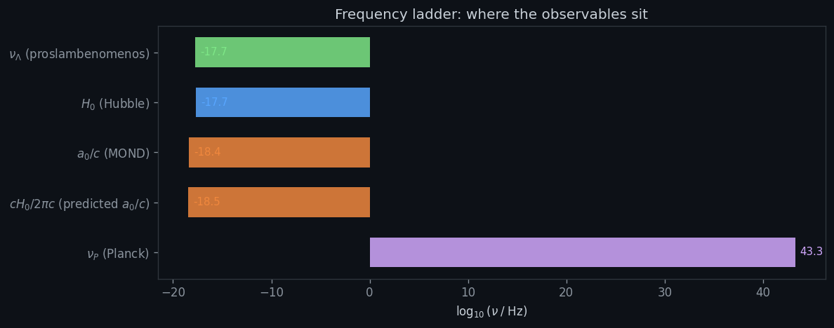
Ratios:
  nu_Lambda / H0      = 0.827647  (framework: sqrt(Omega_Lambda) = 0.827647)
  a0_obs / (cH0/2pi)  = 1.1514
  nu_P / H0           = 8.4919e+60
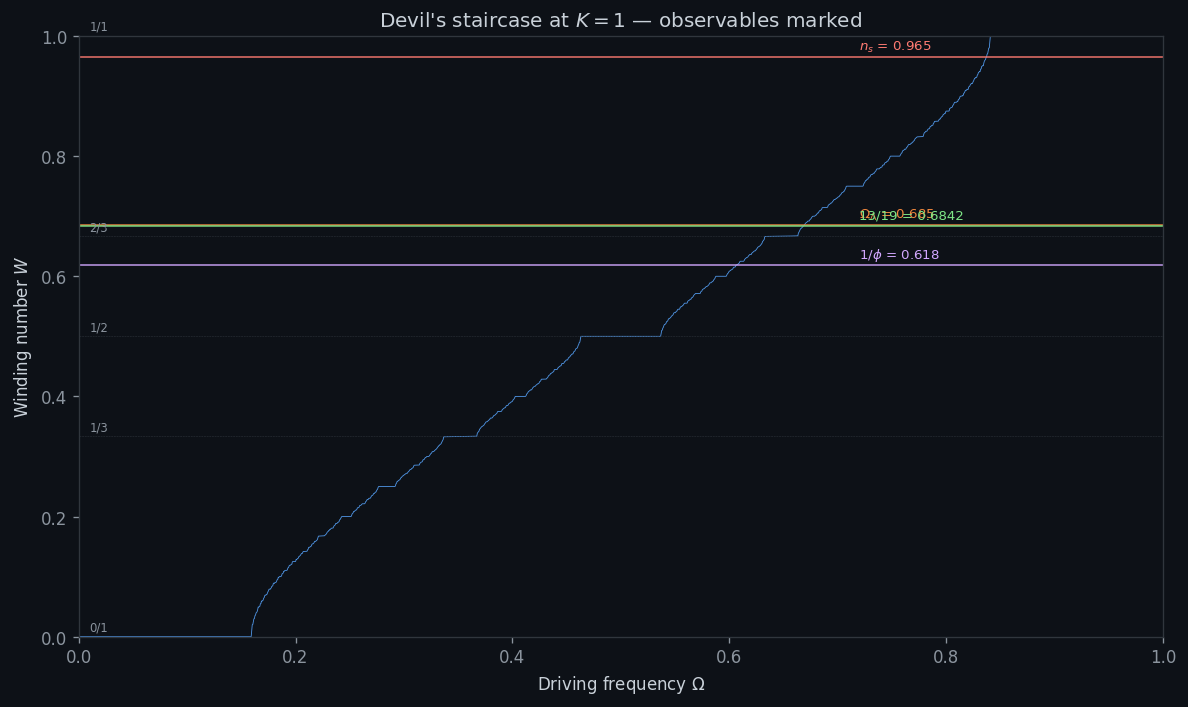
3. The devil’s staircase with observables#
Build the standard circle map staircase and mark where the measured ratios land.
def winding_number(Omega, K, n_iter=200, n_skip=100):
    """Compute winding number of the circle map."""
    theta = 0.0
    for _ in range(n_skip):
        theta = theta + Omega - K / (2 * np.pi) * np.sin(2 * np.pi * theta)
    theta0 = theta
    for _ in range(n_iter):
        theta = theta + Omega - K / (2 * np.pi) * np.sin(2 * np.pi * theta)
    return (theta - theta0) / n_iter

K_crit = 1.0
Omegas = np.linspace(0, 1, 2000)
W = np.array([winding_number(om, K_crit) for om in Omegas])

# Key ratios from observations
phi = (1 + np.sqrt(5)) / 2
observed_ratios = {
    r'$\Omega_\Lambda$ = 0.685': Omega_Lambda_obs,
    '13/19 = 0.6842': 13/19,
    r'$1/\phi$ = 0.618': 1/phi,
    r'$n_s$ = 0.965': n_s_obs,
}

fig, ax = plt.subplots(figsize=(10, 6))
ax.plot(Omegas, W, color='#58a6ff', linewidth=0.5, alpha=0.9)

# Mark tongues for small denominators
for p, q in [(0,1),(1,3),(1,2),(2,3),(1,1)]:
    w_target = p/q if q > 0 else 0
    ax.axhline(w_target, color='#30363d', linewidth=0.3, linestyle='--')
    ax.text(0.01, w_target + 0.01, f'{p}/{q}', fontsize=7, color='#8b949e')

# Plot observed ratios as horizontal markers
colors_obs = ['#f0883e', '#7ee787', '#d2a8ff', '#ff7b72']
for i, (label, val) in enumerate(observed_ratios.items()):
    ax.axhline(val, color=colors_obs[i], linewidth=1.2, linestyle='-', alpha=0.7)
    ax.text(0.72, val + 0.012, label, fontsize=8, color=colors_obs[i])

ax.set_xlabel(r'Driving frequency $\Omega$')
ax.set_ylabel(r'Winding number $W$')
ax.set_title(r"Devil's staircase at $K = 1$ — observables marked")
ax.set_xlim(0, 1)
ax.set_ylim(0, 1)
plt.tight_layout()
plt.show()
4. Stern-Brocot tree: where do the numbers live?#
Every positive rational has a unique address on the Stern-Brocot tree. The depth of that address is the denominator complexity. Plug in the framework’s key rationals and see where they sit.
def stern_brocot_path(p, q, max_depth=30):
    """Find the path from root to p/q on the Stern-Brocot tree.
    Returns list of 'L'/'R' turns and the depth."""
    if q == 0:
        return [], 0
    lo_p, lo_q = 0, 1
    hi_p, hi_q = 1, 0
    path = []
    for _ in range(max_depth):
        med_p = lo_p + hi_p
        med_q = lo_q + hi_q
        if med_p * q == p * med_q:
            return path, len(path)
        elif p * med_q < med_p * q:
            path.append('L')
            hi_p, hi_q = med_p, med_q
        else:
            path.append('R')
            lo_p, lo_q = med_p, med_q
    return path, len(path)

framework_rationals = {
    '1/1 (unity)': (1, 1),
    '1/2': (1, 2),
    '2/3': (2, 3),
    '3/2': (3, 2),
    '13/19 (Omega_Lambda)': (13, 19),
    '|F_6| = 13': (13, 1),
    '54 = exponent': (54, 1),
}

print(f"{'Rational':<25} {'Path':<35} {'Depth'}")
print('-' * 65)
for label, (p, q) in framework_rationals.items():
    path, depth = stern_brocot_path(p, q)
    path_str = ''.join(path) if path else '(root)'
    if len(path_str) > 32:
        path_str = path_str[:29] + '...'
    print(f"{label:<25} {path_str:<35} {depth}")
Rational                  Path                                Depth
-----------------------------------------------------------------
1/1 (unity)               (root)                              0
1/2                       L                                   1
2/3                       LR                                  2
3/2                       RL                                  2
13/19 (Omega_Lambda)      LRRLLLLL                            8
|F_6| = 13                RRRRRRRRRRRR                        12
54 = exponent             RRRRRRRRRRRRRRRRRRRRRRRRRRRRRR      30
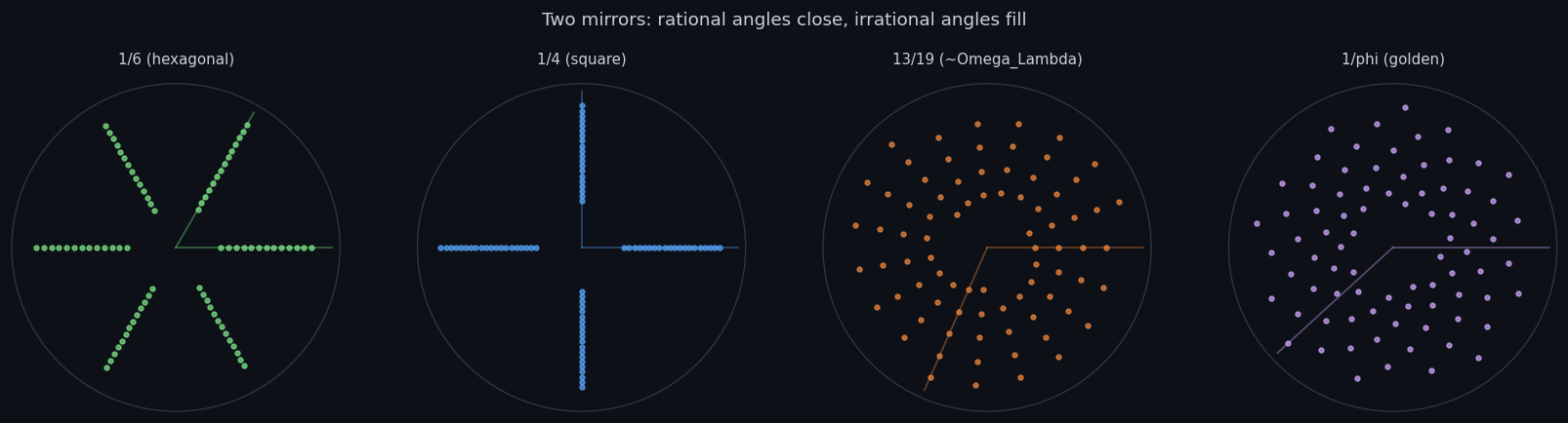
5. The mirrors: recursive image at rational angles#
Two mirrors at angle \(\theta = 2\pi / n\) produce \(n - 1\) reflections. At irrational multiples of \(2\pi\), reflections never close. This is mode-locking on a tabletop.
def mirror_reflections(angle_frac, n_reflections=60):
    """Simulate reflections between two mirrors at angle = angle_frac * 2pi.
    Returns angles of reflected images."""
    angles = []
    for k in range(1, n_reflections + 1):
        # Alternating reflections in two mirrors
        a = k * angle_frac * 2 * np.pi
        a_mod = a % (2 * np.pi)
        angles.append(a_mod)
    return np.array(angles)

fig, axes = plt.subplots(1, 4, figsize=(14, 3.5), subplot_kw={'projection': 'polar'})

cases = [
    ('1/6 (hexagonal)', 1/6, '#7ee787'),
    ('1/4 (square)', 1/4, '#58a6ff'),
    ('13/19 (~Omega_Lambda)', 13/19, '#f0883e'),
    ('1/phi (golden)', 1/phi, '#d2a8ff'),
]

for ax, (title, frac, color) in zip(axes, cases):
    angles = mirror_reflections(frac, n_reflections=80)
    radii = np.linspace(1, 0.3, len(angles))
    ax.scatter(angles, radii, c=color, s=8, alpha=0.7)
    ax.set_title(title, fontsize=9, pad=12)
    ax.set_rticks([])
    ax.set_thetagrids([])
    ax.set_facecolor('#0d1117')
    # Mark the mirror angle
    ax.plot([0, frac * 2 * np.pi], [0, 1.1], color=color, alpha=0.4, linewidth=1)
    ax.plot([0, 0], [0, 1.1], color=color, alpha=0.4, linewidth=1)

fig.suptitle('Two mirrors: rational angles close, irrational angles fill', fontsize=11, y=1.02)
plt.tight_layout()
plt.show()
6. Residuals: framework vs. observation#
No derivation. Just the numbers, side by side.
# Framework values from the derivation chain
a0_predicted = c * H0 / (2 * np.pi)  # D3
Omega_Lambda_pred = 13 / 19           # D25
n_s_pred = 0.965                      # D4 (range: 0.963-0.966)
d_pred = 3                            # D14
d_obs = 3

# Hierarchy ratio D26: R = 6 * 13^54
R_pred = 6 * 13**54
R_obs = nu_P / H0

comparisons = [
    ('Spatial dimensions', d_pred, d_obs, 'exact'),
    ('n_s (spectral tilt)', n_s_pred, n_s_obs, f'{abs(n_s_pred - n_s_obs)/n_s_obs * 100:.2f}%'),
    ('Omega_Lambda', Omega_Lambda_pred, Omega_Lambda_obs, f'{abs(Omega_Lambda_pred - Omega_Lambda_obs)/Omega_Lambda_obs * 100:.2f}%'),
    ('a_0 (m/s^2)', a0_predicted, a0_obs, f'{abs(a0_predicted - a0_obs)/a0_obs * 100:.1f}%'),
    ('log10(nu_P/H0)', np.log10(R_pred), np.log10(R_obs), f'{abs(np.log10(R_pred) - np.log10(R_obs))/np.log10(R_obs) * 100:.2f}%'),
]

fig, ax = plt.subplots(figsize=(10, 4))
ax.axis('off')

headers = ['Observable', 'Framework', 'Measured', 'Residual']
table_data = []
for name, pred, obs, res in comparisons:
    if isinstance(pred, int):
        table_data.append([name, str(pred), str(obs), res])
    else:
        table_data.append([name, f'{pred:.6g}', f'{obs:.6g}', res])

table = ax.table(
    cellText=table_data,
    colLabels=headers,
    loc='center',
    cellLoc='center',
)
table.auto_set_font_size(False)
table.set_fontsize(10)
table.scale(1.0, 1.6)

# Style the table
for (row, col), cell in table.get_celld().items():
    cell.set_edgecolor('#30363d')
    if row == 0:
        cell.set_facecolor('#161b22')
        cell.set_text_props(color='#58a6ff', fontweight='bold')
    else:
        cell.set_facecolor('#0d1117')
        cell.set_text_props(color='#c9d1d9')

ax.set_title('Framework predictions vs. measured values', fontsize=12, pad=20)
plt.tight_layout()
plt.show()

print("\nAll values computed from measured constants (H0, c, G, hbar).")
print("Framework column: what the derivation chain says these should be.")
print("No fitting. No tuning. No free parameters.")
---------------------------------------------------------------------------
AttributeError                            Traceback (most recent call last)
AttributeError: 'int' object has no attribute 'log10'

The above exception was the direct cause of the following exception:

TypeError                                 Traceback (most recent call last)
Cell In[7], line 17
     13     ('Spatial dimensions', d_pred, d_obs, 'exact'),
     14     ('n_s (spectral tilt)', n_s_pred, n_s_obs, f'{abs(n_s_pred - n_s_obs)/n_s_obs * 100:.2f}%'),
     15     ('Omega_Lambda', Omega_Lambda_pred, Omega_Lambda_obs, f'{abs(Omega_Lambda_pred - Omega_Lambda_obs)/Omega_Lambda_obs * 100:.2f}%'),
     16     ('a_0 (m/s^2)', a0_predicted, a0_obs, f'{abs(a0_predicted - a0_obs)/a0_obs * 100:.1f}%'),
---> 17     ('log10(nu_P/H0)', np.log10(R_pred), np.log10(R_obs), f'{abs(np.log10(R_pred) - np.log10(R_obs))/np.log10(R_obs) * 100:.2f}%'),
     18 ]
     19
     20 fig, ax = plt.subplots(figsize=(10, 4))

TypeError: loop of ufunc does not support argument 0 of type int which has no callable log10 method
7. The fidelity question#
How many levels of the Stern-Brocot tree can the universe resolve? The Planck/Hubble ratio sets the answer.
# The number of distinguishable levels
# At each level d of the Stern-Brocot tree, there are 2^d nodes
# The universe can resolve rationals p/q where q is not too large.
# Maximum q ~ nu_P / H0

max_q = nu_P / H0
max_depth_binary = np.log2(max_q)

# The golden ratio's continued fraction is all 1s: [1; 1, 1, 1, ...]
# It takes the maximum number of steps to reach at any given depth
# Depth to approximate phi to precision epsilon: ~ log(1/epsilon) / log(phi)
phi_precision = 1 / max_q
phi_depth = np.log(max_q) / np.log(phi)

print(f"Planck/Hubble ratio:         {max_q:.4e}")
print(f"Binary depth (log2):         {max_depth_binary:.1f} levels")
print(f"Golden-ratio depth:          {phi_depth:.1f} continued-fraction steps")
print(f"Precision at that depth:     {phi_precision:.4e}")
print()
print(f"The spectral tilt n_s = {n_s_obs} deviates from 1 by {1 - n_s_obs:.4f}.")
print(f"This is the tree's finite-depth signature: the recursive image")
print(f"doesn't quite close because the universe has had finite time")
print(f"to traverse the tree.")
print()
print(f"Stern-Brocot levels traversed per Hubble time: ~{max_depth_binary:.0f}")
print(f"Each level doubles the denominator resolution.")
print(f"The spectrum is this many bits deep.")