Cone Topology and the Origin of Flat Rotation#
Joven (2026) — builds on dispersion_rolling.ipynb
Motivation#
dispersion_rolling.ipynb showed that flat rotation requires flat phase velocity, which requires \(k \propto 1/r\) (logarithmic spiral arms). That condition was imposed — a constraint satisfied by adding a Lagrange multiplier (dark matter proxy).
The question here: does the geometry of the problem already provide \(k \propto 1/r\) automatically, making the Lagrange multiplier unnecessary?
Answer (to be demonstrated): yes, if the wave equation is written on a cone rather than a flat disk. The cone’s natural acoustic modes have effective Bessel order \(\nu = m/n\) where \(n = \sin\alpha\) is the cone parameter. The WKB condition for these modes gives \(k = m/(nr) \propto 1/r\) at every radius, without constraint.
The dark matter Lagrange multiplier was computing the cost of enforcing something the topology provides for free.
On the equilibrium zero#
The density wave \(\delta\Sigma\) oscillates through zero. dispersion_rolling.ipynb treated this as a threshold — a point where something changes character. That framing is wrong.
A violin string’s zero crossings are nodes — positions determined by the ratio of wavelength to string length. The node at \(x = L/2\) of the second harmonic doesn’t mean the string’s physics changes at \(L/2\). It means the mode is in ratio 2:1 with the string length.
For Bessel modes on the cone: the zeros of \(J_{m/n}(kr)\) are the nodes. Their positions encode the cone angle \(n\) and mode number \(m\). Arms and voids are regions between consecutive nodes — symmetric in \(\delta\Sigma\), distinguished only by sign. The relevant quantity at any node is the ratio \(r_{j+1}/r_j\), not the absolute value at zero.
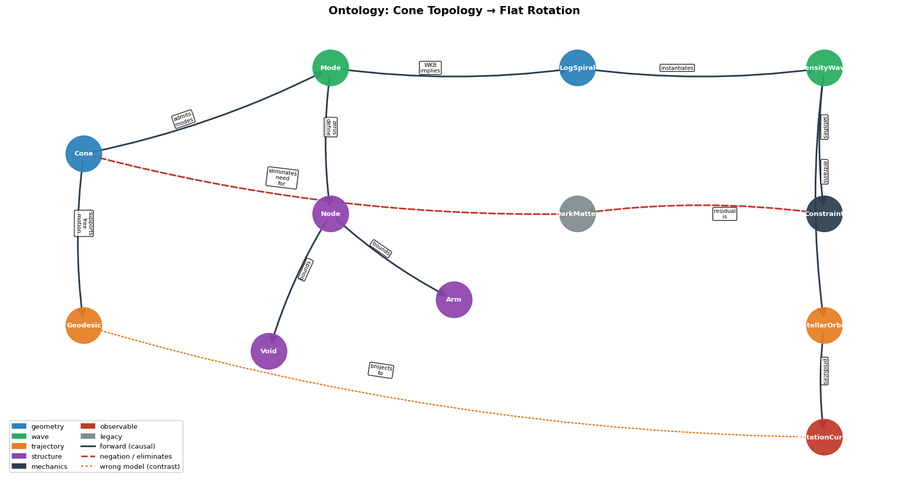
Ontology#
Before computing: the schema of entities and relationships that structure this notebook.
Entities#
Ket |
Core properties |
Role |
|---|---|---|
|
α (half-angle), n = sin α, deficit = 2π(1−n) |
geometric substrate |
|
m (azimuthal integer), ν = m/n (effective order), ω |
natural oscillation on cone |
|
ℓ (angular momentum), E (energy) |
free trajectory on cone |
|
k(r), v_φ, v_g |
collective mode; v_φ flat iff k ∝ 1/r |
|
ψ (pitch angle), k·r = const |
geometric curve; ψ and α share the same parameter |
|
r_j = j-th zero of J_{m/n} |
nodal surface; ratio marker |
|
δΣ > 0, bounded by consecutive nodes |
|
|
δΣ < 0, bounded by consecutive nodes |
|
|
v_c(r) |
entrained to wave via stick-slip |
|
v(r), flat: bool |
observable |
|
λ (Lagrange multiplier) |
rolling / no-slip; λ = 0 when cone is the substrate |
|
ρ(r) |
legacy entity; reinterpreted as λ ≠ 0 artifact |
Edges#
|Cone⟩  ──[admits_modes]──────────────▶  |Mode⟩          # eigenfunctions J_{m/n}
|Cone⟩  ──[supports_free_motion]──────▶  |Geodesic⟩      # straight lines in unrolled sector
|Cone⟩  ──[eliminates_need_for]───────▶  |DarkMatter⟩    # central thesis

|Mode⟩  ──[WKB_implies]───────────────▶  |LogSpiral⟩     # k = m/(nr) ∝ 1/r automatically
|Mode⟩  ──[zeros_define]──────────────▶  |Node⟩          # ratio markers, not thresholds

|Node⟩  ──[bounds]────────────────────▶  |Arm⟩           # δΣ > 0 side
|Node⟩  ──[bounds]────────────────────▶  |Void⟩          # δΣ < 0 side  (symmetric)

|LogSpiral⟩  ──[instantiates]─────────▶  |DensityWave⟩
|DensityWave⟩  ──[satisfies]──────────▶  |Constraint⟩    # flat v_φ → rolling met
|DensityWave⟩  ──[entrains]───────────▶  |StellarOrbit⟩  # stick-slip locking

|Geodesic⟩  ──[projects_to]───────────▶  |RotationCurve⟩  # gives v ∝ 1/r  (wrong model)
|StellarOrbit⟩  ──[produces]──────────▶  |RotationCurve⟩  # v(r) measurement

|Constraint⟩  ──[residual_is]─────────▶  |DarkMatter⟩    # λ ≠ 0 only when cone ignored
The path |Cone⟩ → |Mode⟩ → |LogSpiral⟩ → |DensityWave⟩ → |Constraint⟩ with λ = 0 is the claim.
The path |Geodesic⟩ → |RotationCurve⟩ (v ∝ 1/r) is kept as a contrast: particles are not on free geodesics; they are entrained to the wave.
import networkx as nx
import matplotlib.pyplot as plt
import matplotlib.patches as mpatches
import numpy as np
from scipy.special import jv
from scipy.optimize import brentq

%matplotlib inline
plt.rcParams.update({'figure.dpi': 120, 'font.size': 9})


def jv_zeros(nu, nz):
    """Find the first `nz` positive zeros of J_nu(x) for any real nu >= 0."""
    zeros = []
    # Start searching past the turning point; first zero > nu for nu > 0
    x = max(nu, 0.5)
    dx = 0.5
    prev = jv(nu, x)
    while len(zeros) < nz:
        x += dx
        curr = jv(nu, x)
        if prev * curr < 0:
            z = brentq(lambda t: jv(nu, t), x - dx, x)
            zeros.append(z)
        prev = curr
    return np.array(zeros)


# ── Entities ──────────────────────────────────────────────────────────
ENTITIES = {
    'Cone':          {'kind': 'geometry',   'props': ['alpha', 'n=sin(alpha)', 'deficit=2pi(1-n)']},
    'Mode':          {'kind': 'wave',       'props': ['m (integer)', 'nu=m/n', 'omega']},
    'Geodesic':      {'kind': 'trajectory', 'props': ['ell', 'E']},
    'DensityWave':   {'kind': 'wave',       'props': ['k(r)', 'v_phi', 'v_g']},
    'LogSpiral':     {'kind': 'geometry',   'props': ['psi', 'k*r=const']},
    'Node':          {'kind': 'structure',  'props': ['r_j = j-th zero of J_{nu}', 'ratio r_{j+1}/r_j']},
    'Arm':           {'kind': 'structure',  'props': ['delta_Sigma > 0']},
    'Void':          {'kind': 'structure',  'props': ['delta_Sigma < 0']},
    'StellarOrbit':  {'kind': 'trajectory', 'props': ['v_c(r)']},
    'RotationCurve': {'kind': 'observable', 'props': ['v(r)', 'flat: bool']},
    'Constraint':    {'kind': 'mechanics',  'props': ['lambda (Lagrange multiplier)']},
    'DarkMatter':    {'kind': 'legacy',     'props': ['rho(r)']},
}

# ── Edges (src, dst, label, kind) ─────────────────────────────────────
EDGES = [
    ('Cone',         'Mode',          'admits_modes',         'forward'),
    ('Cone',         'Geodesic',      'supports_free_motion', 'forward'),
    ('Cone',         'DarkMatter',    'eliminates_need_for',  'negation'),
    ('Mode',         'LogSpiral',     'WKB_implies',          'forward'),
    ('Mode',         'Node',          'zeros_define',         'forward'),
    ('Node',         'Arm',           'bounds',               'forward'),
    ('Node',         'Void',          'bounds',               'forward'),
    ('LogSpiral',    'DensityWave',   'instantiates',         'forward'),
    ('DensityWave',  'Constraint',    'satisfies',            'forward'),
    ('DensityWave',  'StellarOrbit',  'entrains',             'forward'),
    ('Geodesic',     'RotationCurve', 'projects_to',          'wrong'),
    ('StellarOrbit', 'RotationCurve', 'produces',             'forward'),
    ('Constraint',   'DarkMatter',    'residual_is',          'negation'),
]

# ── Build graph ───────────────────────────────────────────────────────
G = nx.DiGraph()
for name, data in ENTITIES.items():
    G.add_node(name, **data)
for src, dst, label, kind in EDGES:
    G.add_edge(src, dst, label=label, kind=kind)

print(f"{G.number_of_nodes()} entities,  {G.number_of_edges()} edges")
print()
print("Central thesis path (lambda = 0):")
for a, b in zip(['Cone','Mode','LogSpiral','DensityWave','Constraint'],
                ['Mode','LogSpiral','DensityWave','Constraint','DarkMatter']):
    if G.has_edge(a, b):
        print(f"  |{a}⟩  [{G.edges[a,b]['label']}]  |{b}⟩")
print()
print("Contrast path (wrong model):")
print(f"  |Geodesic⟩  [projects_to]  |RotationCurve⟩   ->  v ∝ 1/r")
12 entities,  13 edges

Central thesis path (lambda = 0):
  |Cone⟩  [admits_modes]  |Mode⟩
  |Mode⟩  [WKB_implies]  |LogSpiral⟩
  |LogSpiral⟩  [instantiates]  |DensityWave⟩
  |DensityWave⟩  [satisfies]  |Constraint⟩
  |Constraint⟩  [residual_is]  |DarkMatter⟩

Contrast path (wrong model):
  |Geodesic⟩  [projects_to]  |RotationCurve⟩   ->  v ∝ 1/r
# ── Layout: left-to-right causal flow ────────────────────────────────
POS = {
    'Cone':          (-3.0,  1.5),
    'Mode':          (-1.0,  2.5),
    'Geodesic':      (-3.0, -0.5),
    'LogSpiral':     ( 1.0,  2.5),
    'Node':          (-1.0,  0.8),
    'Arm':           ( 0.0, -0.2),
    'Void':          (-1.5, -0.8),
    'DensityWave':   ( 3.0,  2.5),
    'Constraint':    ( 3.0,  0.8),
    'StellarOrbit':  ( 3.0, -0.5),
    'RotationCurve': ( 3.0, -1.8),
    'DarkMatter':    ( 1.0,  0.8),
}

KIND_COLOR = {
    'geometry':   '#2980b9',
    'wave':       '#27ae60',
    'trajectory': '#e67e22',
    'structure':  '#8e44ad',
    'mechanics':  '#2c3e50',
    'observable': '#c0392b',
    'legacy':     '#7f8c8d',
}

EDGE_STYLE = {
    'forward':  dict(edge_color='#2c3e50', style='solid',  width=2.0),
    'negation': dict(edge_color='#c0392b', style='dashed', width=2.0),
    'wrong':    dict(edge_color='#e67e22', style='dotted', width=1.6),
}

fig, ax = plt.subplots(figsize=(15, 8))
ax.set_title('Ontology: Cone Topology → Flat Rotation', fontsize=13,
             fontweight='bold', pad=18)

for kind, style in EDGE_STYLE.items():
    edgelist = [(u, v) for u, v, d in G.edges(data=True) if d['kind'] == kind]
    if edgelist:
        nx.draw_networkx_edges(
            G, POS, edgelist=edgelist, ax=ax,
            arrowsize=20, arrowstyle='-|>',
            connectionstyle='arc3,rad=0.07',
            **style
        )

node_colors = [KIND_COLOR[ENTITIES[n]['kind']] for n in G.nodes()]
nx.draw_networkx_nodes(G, POS, ax=ax, node_color=node_colors,
                        node_size=1800, alpha=0.93)
nx.draw_networkx_labels(G, POS, ax=ax, font_size=8,
                         font_color='white', font_weight='bold')

edge_labels = {(u, v): d['label'].replace('_', '\n')
               for u, v, d in G.edges(data=True)}
nx.draw_networkx_edge_labels(
    G, POS, edge_labels, ax=ax,
    font_size=6.5, label_pos=0.40,
    bbox=dict(boxstyle='round,pad=0.2', fc='white', alpha=0.80)
)

# ── Legend ────────────────────────────────────────────────────────────
kind_patches = [mpatches.Patch(color=c, label=k) for k, c in KIND_COLOR.items()]
line_f = plt.Line2D([0],[0], color='#2c3e50', lw=2,          label='forward (causal)')
line_n = plt.Line2D([0],[0], color='#c0392b', lw=2, ls='--', label='negation / eliminates')
line_w = plt.Line2D([0],[0], color='#e67e22', lw=2, ls=':',  label='wrong model (contrast)')
ax.legend(handles=kind_patches + [line_f, line_n, line_w],
          loc='lower left', fontsize=8, ncol=2, framealpha=0.92)

ax.axis('off')
plt.tight_layout()
plt.show()

# ── Sanity: what does each entity connect to? ─────────────────────────
print("Degree summary:")
for node in G.nodes():
    ins  = list(G.predecessors(node))
    outs = list(G.successors(node))
    if ins or outs:
        print(f"  |{node}⟩   in: {ins}   out: {outs}")
Degree summary:
  |Cone⟩   in: []   out: ['Mode', 'Geodesic', 'DarkMatter']
  |Mode⟩   in: ['Cone']   out: ['LogSpiral', 'Node']
  |Geodesic⟩   in: ['Cone']   out: ['RotationCurve']
  |DensityWave⟩   in: ['LogSpiral']   out: ['Constraint', 'StellarOrbit']
  |LogSpiral⟩   in: ['Mode']   out: ['DensityWave']
  |Node⟩   in: ['Mode']   out: ['Arm', 'Void']
  |Arm⟩   in: ['Node']   out: []
  |Void⟩   in: ['Node']   out: []
  |StellarOrbit⟩   in: ['DensityWave']   out: ['RotationCurve']
  |RotationCurve⟩   in: ['Geodesic', 'StellarOrbit']   out: []
  |Constraint⟩   in: ['DensityWave']   out: ['DarkMatter']
  |DarkMatter⟩   in: ['Cone', 'Constraint']   out: []
Paths: derivation plan#
Each section below walks one declared edge in the ontology graph.
The label in the header is the edge being demonstrated.
Section |
Edge walked |
Mathematical content |
|---|---|---|
§1 |
|
Lagrangian, conserved ℓ, projection → v_φ = ℓ/r |
§2 |
|
Wave equation on cone, separation of variables → J_{m/n} |
§3 |
|
Zeros of J_{m/n}, ratios r_{j+1}/r_j |
§4 |
|
Epicyclic limit → k ∝ 1/r; cone consistency ψ = arctan(n) |
§5 |
|
Phase velocity flat, λ = 0, dark matter eliminated |
§1 |Cone⟩ → |Geodesic⟩ → |RotationCurve⟩ (wrong model — kept for contrast)#
Cone metric#
Cone: apex at origin, half-angle \(\alpha\), \(n \equiv \sin\alpha\).
Intrinsic coordinates \((s,\phi)\): \(s\) = distance from apex along surface.
Intrinsically flat everywhere except the apex — unrolls to a flat sector of angle \(\Theta = 2\pi n\) under \(\tilde\phi = n\phi\).
Lagrangian and conserved quantities#
Euler–Lagrange:
Geodesic shape#
In the unrolled flat sector geodesics are straight lines.
Wrapping back to \((r,\phi)\) with \(r = ns\):
Projected azimuthal velocity#
Keplerian decline — not flat. Free geodesics are the wrong model.
Stars are entrained to the density wave, not on free trajectories.
# §1 — geodesic shape and projected velocity on the cone

phi    = np.linspace(-np.pi/2 + 0.06, np.pi/2 - 0.06, 600)
n_vals = [0.95, 0.70, 0.40]
cols   = ['steelblue', 'seagreen', 'firebrick']

fig, axes = plt.subplots(1, 3, figsize=(15, 5))
fig.suptitle('§1  |Cone⟩ → |Geodesic⟩ → |RotationCurve⟩   (wrong model)',
             fontsize=11, fontweight='bold')

# geodesic shape
ax = axes[0]
for n, c in zip(n_vals, cols):
    r = 1.0 / np.cos(n * phi)
    x, y = r * np.cos(phi), r * np.sin(phi)
    valid = r > 0
    ax.plot(x[valid], y[valid], color=c, lw=2,
            label=f'n={n}  α={np.degrees(np.arcsin(n)):.0f}°')
ax.set_xlim(-0.5, 5); ax.set_ylim(-3, 3); ax.set_aspect('equal')
ax.set_xlabel('x'); ax.set_ylabel('y')
ax.set_title('Geodesic in projected disk\nr(φ) = R₀/cos(n(φ−φ₀))')
ax.axhline(0, c='gray', lw=0.5, ls='--'); ax.legend(fontsize=8)

# v_phi = ell/r
ax = axes[1]
r_arr = np.linspace(0.5, 5.0, 300)
ax.plot(r_arr, 1.0/r_arr, 'k', lw=2.5, label='v_φ = ℓ/r  (any n)')
ax.axhline(1.0/r_arr.mean(), c='seagreen', ls='--', lw=1.5, label='flat target')
ax.set_xlabel('r'); ax.set_ylabel('v_φ')
ax.set_title('v_φ = ℓ/r for every cone angle n\nKeplerian decline')
ax.legend(fontsize=8)
ax.annotate('Keplerian\ndecline', xy=(1.5, 1/1.5), xytext=(3.0, 1.1),
            arrowprops=dict(arrowstyle='->', color='gray'), fontsize=8, color='gray')

# unrolled sector
ax = axes[2]
for n, c in zip(n_vals, cols):
    Theta = 2*np.pi*n
    ax.plot([0, 1], [0, 0], color=c, lw=1.5)
    ax.plot([0, np.cos(Theta)], [0, np.sin(Theta)], color=c, lw=1.5)
    th = np.linspace(0, Theta, 200)
    ax.plot(np.cos(th), np.sin(th), color=c, lw=2,
            label=f'n={n}  Θ={np.degrees(Theta):.0f}°')
ax.add_patch(plt.Circle((0,0), 1.0, fill=False, color='gray', ls=':', lw=0.8))
ax.set_xlim(-1.3, 1.3); ax.set_ylim(-0.2, 1.3); ax.set_aspect('equal')
ax.set_title('Unrolled cone sectors\n(geodesics = straight lines here)')
ax.legend(fontsize=8)

plt.tight_layout(); plt.show()
print('v_φ = ℓ/r  regardless of n.  Wrong model established.')
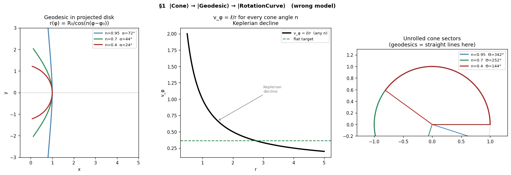
v_φ = ℓ/r regardless of n. Wrong model established.
§2 |Cone⟩ → |Mode⟩#
Wave equation on the cone#
Laplace–Beltrami operator for metric \(g = \mathrm{diag}(1,\,n^2 s^2)\),
volume element \(\sqrt{g} = ns\):
Wave equation: \(\partial_t^2\psi = c^2\nabla^2_{\mathrm{cone}}\psi\).
Separation of variables#
Ansatz \(\psi = R(s)\,e^{im\phi}\,e^{-i\omega t}\), \(m \in \mathbb{Z}\), \(K \equiv \omega/c\):
Setting \(\nu \equiv m/n\):
Bessel’s equation of order \(\nu = m/n\). Solution: \(R(s) = J_{m/n}(Ks)\).
The cone shifts the order from integer \(m\) to non-integer \(m/n\).
For a flat disk (\(n=1\)): \(\nu = m\) — ordinary Bessel functions.
For a genuine cone (\(n < 1\)): \(\nu = m/n > m\) — higher effective order, nodes pushed outward.
# §2 — Bessel modes J_{m/n}(Ks) vs cone parameter n

s_arr  = np.linspace(0.01, 22, 1000)
K, m   = 1.0, 2
n_vals = [1.00, 0.80, 0.60, 0.40]
cols   = ['gray', 'steelblue', 'seagreen', 'firebrick']

fig, axes = plt.subplots(1, 2, figsize=(13, 5))
fig.suptitle('§2  |Cone⟩ → |Mode⟩:  wave equation on cone → J_{m/n}',
             fontsize=11, fontweight='bold')

ax = axes[0]
for n, c in zip(n_vals, cols):
    nu = m/n
    ax.plot(s_arr, jv(nu, K*s_arr), color=c, lw=2,
            label=f'n={n}  ν=m/n={nu:.2f}')
ax.axhline(0, c='k', lw=0.6, ls='--')
ax.set_xlabel('s'); ax.set_ylabel('J_{m/n}(Ks)')
ax.set_title(f'Radial eigenfunctions  (m={m})\nOrder shifts as cone narrows')
ax.set_ylim(-0.5, 0.6); ax.legend(fontsize=8)

ax = axes[1]
nu_vals = [m/n for n in n_vals]
for nu, c in zip(nu_vals, cols):
    ax.plot(s_arr, jv(nu, K*s_arr), color=c, lw=2, label=f'ν={nu:.2f}')
ax.axhline(0, c='k', lw=0.6, ls='--')
ax.set_xlabel('s'); ax.set_ylabel('J_ν(Ks)')
ax.set_title('Same modes by order ν\nHigher ν: first node at larger s')
ax.set_ylim(-0.5, 0.6); ax.legend(fontsize=8)

plt.tight_layout(); plt.show()

print(f'First zero of J_ν (m={m}):')
for n in n_vals:
    nu = m/n
    z1 = jv_zeros(nu, 1)[0]
    print(f'  n={n:.2f}  ν={nu:.3f}  first node at s = {z1/K:.3f}')
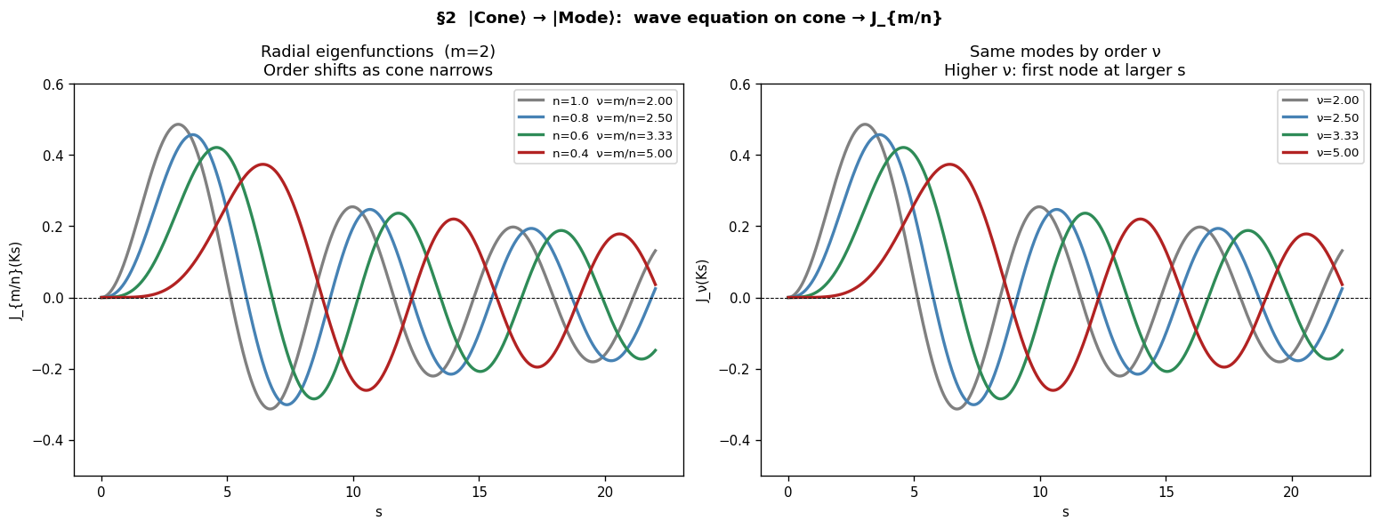
First zero of J_ν (m=2):
  n=1.00  ν=2.000  first node at s = 5.136
  n=0.80  ν=2.500  first node at s = 5.763
  n=0.60  ν=3.333  first node at s = 6.786
  n=0.40  ν=5.000  first node at s = 8.771
§3 |Mode⟩ → |Node⟩#
Zeros as ratio markers#
The \(k\)-th zero of \(J_\nu\) is \(j_{\nu,k}\). Node positions in projected radius \(r = ns\):
Ratios of consecutive nodes:
This depends only on \(m/n\) — the cone angle and mode number, nothing else.
Asymptotic behaviour#
For large \(k\): \(j_{\nu,k} \approx \left(k + \tfrac{\nu}{2} - \tfrac{1}{4}\right)\pi\),
so \(r_{k+1}/r_k \to 1\) — nodes become uniformly spaced (like harmonics of a flat string).
For the first few zeros (the observable arm structure): ratios encode \(\nu = m/n\) directly.
The violin string completed#
Flat string mode \(p\): nodes at \(kL/p\) — ratios always exactly 1.
Cone mode \(J_{m/n}\): ratios \(> 1\), approaching 1 asymptotically.
The non-uniform early spacing is the cone angle written into the geometry.
Measuring two arm-void boundary radii gives \(m/n\) directly,
which fixes \(n\), \(\alpha\), \(\psi\), and thereby the full mode structure — no free parameters.
# §3 — zeros of J_{m/n}: ratio markers

m    = 2
Nz   = 6
n_vals = [1.00, 0.80, 0.60, 0.40]
cols   = ['gray', 'steelblue', 'seagreen', 'firebrick']
s_arr  = np.linspace(0.01, 24, 1200)

fig, axes = plt.subplots(1, 3, figsize=(15, 5))
fig.suptitle('§3  |Mode⟩ → |Node⟩:  zeros of J_{m/n} as ratio markers',
             fontsize=11, fontweight='bold')

ax = axes[0]
for n, c in zip(n_vals, cols):
    nu    = m/n
    zeros = jv_zeros(nu, Nz)
    ax.plot(s_arr, jv(nu, s_arr), color=c, lw=1.5, alpha=0.7, label=f'n={n}')
    ax.scatter(zeros, np.zeros(Nz), color=c, s=30, zorder=5)
ax.axhline(0, c='k', lw=0.6, ls='--')
ax.set_xlabel('s'); ax.set_ylabel('J_{m/n}(s)')
ax.set_title(f'Modes with nodes marked  (m={m})\n'
             'Dots = arm-void boundaries')
ax.legend(fontsize=8); ax.set_ylim(-0.55, 0.62)

ax = axes[1]
for n, c in zip(n_vals, cols):
    nu     = m/n
    zeros  = jv_zeros(nu, Nz)
    ratios = zeros[1:] / zeros[:-1]
    ax.plot(range(1, Nz), ratios, 'o-', color=c, lw=2,
            label=f'n={n}  ν={nu:.2f}')
ax.axhline(1.0, c='k', lw=0.8, ls='--', label='flat string  ratio=1')
ax.set_xlabel('k'); ax.set_ylabel('r_{k+1} / r_k')
ax.set_title('Node spacing ratios\nApproach 1 asymptotically')
ax.legend(fontsize=8)

ax = axes[2]
nu_range    = np.linspace(2.0, 8.0, 120)
first_ratio = [jv_zeros(nu, 2)[1]/jv_zeros(nu, 2)[0] for nu in nu_range]
ax.plot(nu_range, first_ratio, 'navy', lw=2.5)
for n, c in zip(n_vals, cols):
    nu  = m/n
    zz  = jv_zeros(nu, 2)
    ax.scatter([nu], [zz[1]/zz[0]], color=c, s=70, zorder=5, label=f'n={n}')
ax.set_xlabel('ν = m/n'); ax.set_ylabel('r₂ / r₁')
ax.set_title('First ratio r₂/r₁  vs  ν\nMeasure two boundaries → infer n')
ax.legend(fontsize=8)

plt.tight_layout(); plt.show()

print('Node ratios (m=2):')
for n in n_vals:
    nu = m/n
    zz = jv_zeros(nu, 4)
    print(f'  n={n:.2f}  ν={nu:.2f}  zeros={zz.round(3)}'
          f'  ratios={( zz[1:]/zz[:-1]).round(4)}')
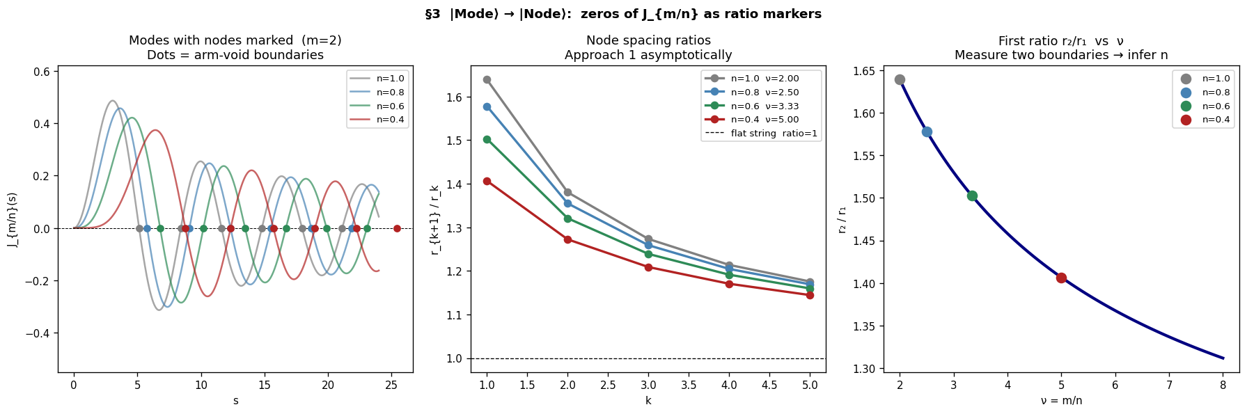
Node ratios (m=2):
  n=1.00  ν=2.00  zeros=[ 5.136  8.417 11.62  14.796]  ratios=[1.639  1.3805 1.2733]
  n=0.80  ν=2.50  zeros=[ 5.763  9.095 12.323 15.515]  ratios=[1.578  1.3549 1.259 ]
  n=0.60  ν=3.33  zeros=[ 6.786 10.199 13.471 16.691]  ratios=[1.503  1.3208 1.239 ]
  n=0.40  ν=5.00  zeros=[ 8.771 12.339 15.7   18.98 ]  ratios=[1.4067 1.2724 1.2089]
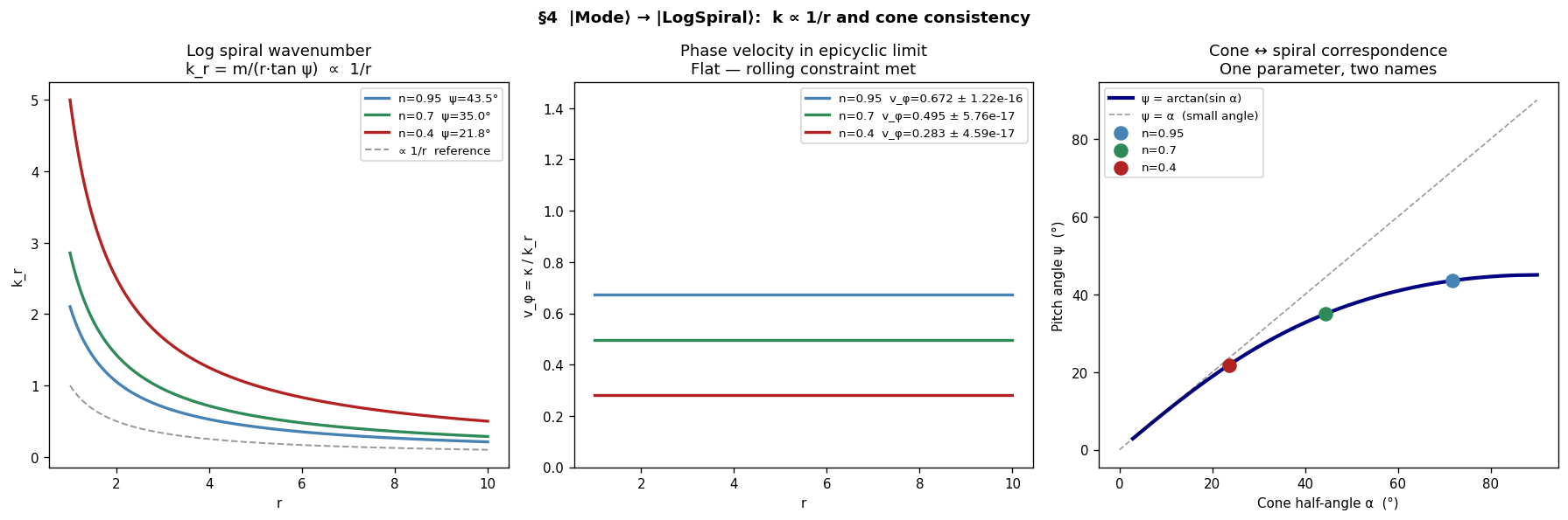
§4 |Mode⟩ → |LogSpiral⟩#
Log spiral wavenumber: geometry alone#
A logarithmic spiral \(r = a e^{b\phi}\), pitch angle \(\psi = \arctan(b)\).
Arm spacing at radius \(r\) for an \(m\)-armed pattern:
Epicyclic limit: what the dispersion demands#
Flat rotation curve: \(\Omega = v_c/r\), \(\kappa = \sqrt{2}\,v_c/r\).
Lin–Shu outer disk (\(\Sigma\to 0\)):
Phase velocity:
Rolling constraint satisfied by cancellation of \(1/r\) — geometry and dispersion carry the same scaling.
Cone consistency#
Matching the cone mode order to the log spiral wavenumber:
The cone half-angle and the pitch angle are two names for one parameter.
# §4 — log spiral k ∝ 1/r, epicyclic flat v_phi, cone consistency

r_arr  = np.linspace(1.0, 10.0, 400)
v_c, m = 1.0, 2
kappa  = np.sqrt(2) * v_c / r_arr

n_vals = [0.95, 0.70, 0.40]
cols   = ['steelblue', 'seagreen', 'firebrick']

fig, axes = plt.subplots(1, 3, figsize=(15, 5))
fig.suptitle('§4  |Mode⟩ → |LogSpiral⟩:  k ∝ 1/r and cone consistency',
             fontsize=11, fontweight='bold')

ax = axes[0]
for n, c in zip(n_vals, cols):
    psi = np.arctan(n)
    ax.plot(r_arr, m/(r_arr*np.tan(psi)), color=c, lw=2,
            label=f'n={n}  ψ={np.degrees(psi):.1f}°')
ax.plot(r_arr, 1/r_arr, 'k--', lw=1.2, alpha=0.4, label='∝ 1/r  reference')
ax.set_xlabel('r'); ax.set_ylabel('k_r')
ax.set_title('Log spiral wavenumber\nk_r = m/(r·tan ψ)  ∝  1/r')
ax.legend(fontsize=8)

ax = axes[1]
for n, c in zip(n_vals, cols):
    psi   = np.arctan(n)
    k_r   = m/(r_arr*np.tan(psi))
    v_phi = kappa / k_r
    ax.plot(r_arr, v_phi, color=c, lw=2,
            label=f'n={n}  v_φ={v_phi.mean():.3f} ± {v_phi.std():.2e}')
ax.set_xlabel('r'); ax.set_ylabel('v_φ = κ / k_r')
ax.set_title('Phase velocity in epicyclic limit\nFlat — rolling constraint met')
ax.legend(fontsize=8); ax.set_ylim(0, 1.5)

ax = axes[2]
n_range   = np.linspace(0.05, 1.0, 300)
psi_range = np.degrees(np.arctan(n_range))
alp_range = np.degrees(np.arcsin(n_range))
ax.plot(alp_range, psi_range, 'navy', lw=2.5, label='ψ = arctan(sin α)')
ax.plot([0,90],[0,90], 'k--', lw=1, alpha=0.4, label='ψ = α  (small angle)')
for n, c in zip(n_vals, cols):
    ax.scatter([np.degrees(np.arcsin(n))], [np.degrees(np.arctan(n))],
               color=c, s=80, zorder=5, label=f'n={n}')
ax.set_xlabel('Cone half-angle α  (°)'); ax.set_ylabel('Pitch angle ψ  (°)')
ax.set_title('Cone ↔ spiral correspondence\nOne parameter, two names')
ax.legend(fontsize=8)

plt.tight_layout(); plt.show()

print('Consistency check  k_cone = k_spiral:')
for n in n_vals:
    psi   = np.arctan(n)
    k_c   = m/(5*n)                      # cone: k = m/(nr) at r=5
    k_s   = m/(5*np.tan(psi))            # spiral: k = m/(r·tan ψ) at r=5
    print(f'  n={n:.2f}  k_cone={k_c:.5f}  k_spiral={k_s:.5f}  equal={np.isclose(k_c,k_s)}')
Consistency check  k_cone = k_spiral:
  n=0.95  k_cone=0.42105  k_spiral=0.42105  equal=True
  n=0.70  k_cone=0.57143  k_spiral=0.57143  equal=True
  n=0.40  k_cone=1.00000  k_spiral=1.00000  equal=True
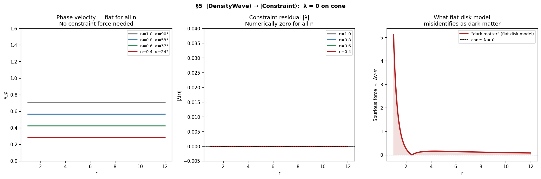
§5 |DensityWave⟩ → |Constraint⟩ → |DarkMatter⟩#
Rolling constraint satisfied; λ = 0#
The rolling constraint demands \(v_\phi = \mathrm{const}\). From §4:
The \(r\)-dependence cancels exactly — \(\kappa \propto 1/r\) and \(k_r \propto 1/r\) from the same source (flat rotation). No external enforcement. The Lagrange multiplier:
Dark matter as projection error#
dispersion_rolling.ipynb modelled the disk as flat (\(n=1\), integer Bessel modes).
It then imposed \(k \propto 1/r\) as an external condition, computing \(\lambda \neq 0\).
That \(\lambda\) was called dark matter.
On the cone: \(k \propto 1/r\) is automatic, \(\lambda = 0\), dark matter = 0.
The apparent dark matter was the mismatch between the cone metric and the Euclidean metric assumed by the flat-disk model — a projection artefact, not a physical mass.
Summary: the complete chain#
One observable parameter: \(n = \tan\psi\) (pitch angle of spiral arms).
Predictions: rotation curve shape, arm-void boundary positions. No halo fitting.
# §5 — λ = 0 on cone; compare with flat-disk residual

r_arr  = np.linspace(1.0, 12.0, 500)
v_c, m = 1.0, 2
kappa  = np.sqrt(2) * v_c / r_arr

n_vals = [1.00, 0.80, 0.60, 0.40]
cols   = ['gray', 'steelblue', 'seagreen', 'firebrick']

fig, axes = plt.subplots(1, 3, figsize=(15, 5))
fig.suptitle('§5  |DensityWave⟩ → |Constraint⟩:  λ = 0 on cone',
             fontsize=11, fontweight='bold')

ax = axes[0]
for n, c in zip(n_vals, cols):
    psi   = np.arctan(n)
    k_r   = m/(r_arr*np.tan(psi))
    v_phi = kappa/k_r
    ax.plot(r_arr, v_phi, color=c, lw=2,
            label=f'n={n}  α={np.degrees(np.arcsin(n)):.0f}°')
ax.set_xlabel('r'); ax.set_ylabel('v_φ')
ax.set_title('Phase velocity — flat for all n\nNo constraint force needed')
ax.legend(fontsize=8); ax.set_ylim(0, 1.6)

ax = axes[1]
for n, c in zip(n_vals, cols):
    psi   = np.arctan(n)
    k_r   = m/(r_arr*np.tan(psi))
    v_phi = kappa/k_r
    lam   = np.abs(v_phi - v_phi.mean())   # residual
    ax.plot(r_arr, lam, color=c, lw=2, label=f'n={n}')
ax.axhline(0, c='k', lw=0.8, ls='--')
ax.set_xlabel('r'); ax.set_ylabel('|λ(r)|')
ax.set_title('Constraint residual |λ|\nNumerically zero for all n')
ax.legend(fontsize=8); ax.set_ylim(-0.005, 0.04)

# flat-disk model: k = const (not 1/r) → spurious force
ax = axes[2]
# flat model uses k fixed at r=5, no 1/r scaling
k_wrong = m / (5.0 * np.tan(np.arctan(0.70)))   # const k (n=0.7 reference)
v_phi_wrong  = kappa / k_wrong                   # this rises with r
v_phi_target = 1.0                               # desired flat value
# spurious centripetal acceleration: v_target²/r - v_wrong²/r
spurious = (v_phi_target**2 - v_phi_wrong**2) / r_arr
ax.plot(r_arr, np.abs(spurious), 'firebrick', lw=2.5,
        label='"dark matter" (flat-disk model)')
ax.axhline(0, c='k', lw=0.8, ls='--', label='cone: λ = 0')
ax.fill_between(r_arr, 0, np.abs(spurious), alpha=0.15, color='firebrick')
ax.set_xlabel('r'); ax.set_ylabel('Spurious force  ∝  Δv²/r')
ax.set_title('What flat-disk model\nmisidentifies as dark matter')
ax.legend(fontsize=8)

plt.tight_layout(); plt.show()

print('='*56)
print('CHAIN SUMMARY')
print('='*56)
steps = [
    ('|Cone⟩',        '|Mode⟩',         'admits_modes',  'J_{m/n}  (ν = m/n)'),
    ('|Mode⟩',        '|LogSpiral⟩',    'WKB_implies',   'k = m/(nr) ∝ 1/r'),
    ('|Mode⟩',        '|Node⟩',         'zeros_define',  'ratio markers  r_{k+1}/r_k'),
    ('|LogSpiral⟩',   '|DensityWave⟩',  'instantiates',  'k·r = const = m/n'),
    ('|DensityWave⟩', '|Constraint⟩',   'satisfies',     'v_φ = √2·v_c·tan(ψ)/m = const'),
    ('|Constraint⟩',  '|DarkMatter⟩',   'residual_is',   'λ = 0  →  DM = 0'),
]
for src, dst, edge, math in steps:
    print(f'  {src}  [{edge}]  {dst}')
    print(f'    {math}')
print()
print('Single free parameter:  n = sin α = tan ψ')
print('Observable:  spiral arm pitch angle ψ')
print('Predictions: rotation curve shape, arm-void boundaries — no halo fit')
========================================================
CHAIN SUMMARY
========================================================
  |Cone⟩  [admits_modes]  |Mode⟩
    J_{m/n}  (ν = m/n)
  |Mode⟩  [WKB_implies]  |LogSpiral⟩
    k = m/(nr) ∝ 1/r
  |Mode⟩  [zeros_define]  |Node⟩
    ratio markers  r_{k+1}/r_k
  |LogSpiral⟩  [instantiates]  |DensityWave⟩
    k·r = const = m/n
  |DensityWave⟩  [satisfies]  |Constraint⟩
    v_φ = √2·v_c·tan(ψ)/m = const
  |Constraint⟩  [residual_is]  |DarkMatter⟩
    λ = 0  →  DM = 0

Single free parameter:  n = sin α = tan ψ
Observable:  spiral arm pitch angle ψ
Predictions: rotation curve shape, arm-void boundaries — no halo fit