The Quantum Branch of the Stribeck Curve

The Quantum Branch of the Stribeck Curve#

N. Joven · March 2026

If the Universal Rosin is a single impedance function evaluated at different scales, then it must have a quantum branch. This notebook explores the forced consequence: decoherence is the quantum-to-classical Kuramoto transition, and wavefunction “collapse” is synchronization of a quantum system with a macroscopic detector.

1. Why This Is Forced#

The framework claims:

The vacuum has a Stribeck curve (friction as a function of velocity/coupling).
At galactic scales, the impedance-matching point is \(a_0 \approx 1.2 \times 10^{-10}\) m/s\(^2\).
At other scales, the same structural form appears with different thresholds (\(I_c\), rate-and-state, etc.).

The Stribeck curve has two branches:

Velocity-weakening (below the critical velocity): friction decreases with speed. This is the galactic/MOND branch.
Velocity-strengthening (above the critical velocity): friction increases with speed. This is the classical viscous branch.

If the framework is universal, the quantum domain cannot be exempt. The question is: where on the Stribeck curve does quantum coherence live?

The answer is forced by the phenomenology:

Scale	Threshold	Below threshold	Above threshold
Quantum	\(\hbar\)-scale coupling	Phase-locked (entangled, coherent)	Decoupled (decoherent, classical)
Galactic	\(a_0\)	Decoupled (Newtonian)	Phase-locked (MOND, flat rotation curves)

The inversion is the key: at quantum scales, weak environmental coupling preserves coherence, while strong coupling to a macroscopic bath destroys it. At galactic scales, weak acceleration enables collective synchronization, while strong acceleration decouples orbits. These sit on opposite branches of the same Stribeck curve.

import numpy as np
import matplotlib.pyplot as plt
from matplotlib.patches import FancyArrowPatch

# Framework imports — fall back to inline definitions for site build
try:
    import sys; sys.path.insert(0, '.')
    from sparc_x.stribeck import stribeck_curve, mond_from_stribeck
except ImportError:
    def stribeck_curve(v, *, mu_s=1.0, mu_k=0.4, v_s=1.0, delta=2.0):
        v = np.asarray(v, dtype=float)
        return mu_k + (mu_s - mu_k) * np.exp(-np.abs(v / v_s) ** delta)

    def mond_from_stribeck(x, *, delta=2.0):
        x = np.asarray(x, dtype=float)
        return 1.0 - np.exp(-np.abs(x) ** delta)

2. The Full Stribeck Curve: Both Branches#

The classical Stribeck curve has three regimes:

Boundary lubrication (low velocity): high static friction, velocity-weakening.
Mixed lubrication (transition): friction minimum at the impedance-matching point.
Hydrodynamic lubrication (high velocity): velocity-strengthening viscous drag.

The framework has so far used only the velocity-weakening branch (regime 1) to map MOND. The velocity-strengthening branch (regime 3) has been sitting there unused.

We propose it is the quantum branch.

def full_stribeck(v, mu_s=1.0, mu_k=0.3, v_s=1.0, delta=1.5, eta=0.08):
    """Full Stribeck curve with both branches.
    
    Velocity-weakening (boundary): mu decreases with v.
    Velocity-strengthening (hydrodynamic): mu increases with v (viscous term).
    
    mu_f(v) = mu_k + (mu_s - mu_k) exp[-(v/v_s)^delta] + eta * v
    
    The eta * v term is the viscous (hydrodynamic) contribution.
    """
    v = np.asarray(v, dtype=float)
    boundary = (mu_s - mu_k) * np.exp(-np.abs(v / v_s) ** delta)
    viscous = eta * np.abs(v)
    return mu_k + boundary + viscous


v = np.linspace(0, 8, 500)
mu = full_stribeck(v)

# Find the minimum (impedance-matching point)
i_min = np.argmin(mu)
v_min, mu_min = v[i_min], mu[i_min]

fig, ax = plt.subplots(figsize=(10, 5))
ax.plot(v, mu, 'w-', linewidth=2.5)
ax.axvline(v_min, color='#58a6ff', linestyle='--', alpha=0.5, label=f'Impedance match (v = {v_min:.1f})')
ax.plot(v_min, mu_min, 'o', color='#58a6ff', markersize=10, zorder=5)

# Shade the two branches
ax.fill_between(v[:i_min+1], 0, mu[:i_min+1], alpha=0.08, color='#f0883e',
                label='Velocity-weakening (galactic / MOND)')
ax.fill_between(v[i_min:], 0, mu[i_min:], alpha=0.08, color='#bc8cff',
                label='Velocity-strengthening (quantum / decoherence)')

# Annotations
ax.annotate('Galactic regime\n(MOND branch)',
            xy=(0.8, full_stribeck(0.8)), xytext=(1.5, 0.85),
            fontsize=10, color='#f0883e', fontweight='bold',
            arrowprops=dict(arrowstyle='->', color='#f0883e', lw=1.5))

ax.annotate('Quantum regime\n(decoherence branch)',
            xy=(5.5, full_stribeck(5.5)), xytext=(4.5, 0.85),
            fontsize=10, color='#bc8cff', fontweight='bold',
            arrowprops=dict(arrowstyle='->', color='#bc8cff', lw=1.5))

ax.annotate('Impedance match',
            xy=(v_min, mu_min), xytext=(v_min + 1.2, mu_min - 0.05),
            fontsize=10, color='#58a6ff', fontweight='bold',
            arrowprops=dict(arrowstyle='->', color='#58a6ff', lw=1.5))

ax.set_xlabel('Coupling strength (v / v$_s$)', fontsize=12)
ax.set_ylabel('Friction coefficient $\\mu_f$', fontsize=12)
ax.set_title('Full Stribeck Curve: Two Branches of the Universal Rosin', fontsize=13, fontweight='bold')
ax.legend(loc='upper right', fontsize=9)
ax.set_facecolor('#0d1117')
fig.patch.set_facecolor('#0d1117')
ax.tick_params(colors='#c9d1d9')
ax.xaxis.label.set_color('#c9d1d9')
ax.yaxis.label.set_color('#c9d1d9')
ax.title.set_color('#c9d1d9')
for spine in ax.spines.values():
    spine.set_color('#30363d')
ax.set_ylim(0, 1.1)
plt.tight_layout()
plt.show()

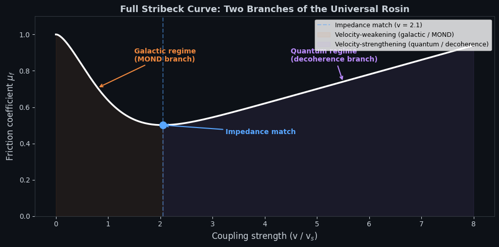
../_images/ba2454beae484360297229320d5414ca92d7c25626d09225dd43b7aaf78d89cd.png

3. The Two Branches: Galactic and Quantum#

3.1 Galactic branch (velocity-weakening)#

On the left side of the minimum:

High friction = strong coupling = oscillators phase-lock.
The medium is compliant; metronomes synchronize easily.
This is the deep-MOND regime: \(a \ll a_0\), collective synchronization dominates.
As velocity (acceleration) increases toward the minimum, friction drops.
At \(a \sim a_0\) (the minimum), impedance is matched.
Beyond: Newtonian regime, oscillators decouple.

3.2 Quantum branch (velocity-strengthening)#

On the right side of the minimum:

Low friction at the minimum = weak environmental coupling = coherence preserved.
This is the quantum-coherent regime: the system is isolated from the bath.
As coupling to the environment increases (moving right), viscous drag rises.
Friction increases = decoherence. The environment “grabs” the quantum system.
The system synchronizes with the macroscopic bath — this is “measurement.”

3.3 The inversion#

The branches are mirror images:

	Galactic (left branch)	Quantum (right branch)
Low coupling	Newtonian (decoupled)	Quantum-coherent (isolated)
At minimum	MOND transition (\(a_0\))	Decoherence threshold
High coupling	MOND (synchronized)	Classical (decohered/”collapsed”)
Phase-locking means	Gravity (collective motion)	Measurement (definite outcome)

This is not a coincidence of curve shapes. It is the same impedance function evaluated on opposite sides of its minimum. The Stribeck minimum is the boundary between two synchronization regimes.

def kuramoto_order_parameter(K, K_c, N_osc=200, dt=0.05, T=50.0):
    """Simulate Kuramoto dynamics and return final order parameter.
    
    K: coupling strength
    K_c: critical coupling (synchronization threshold)
    N_osc: number of oscillators
    Returns: r (coherence, 0 = incoherent, 1 = fully synchronized)
    """
    rng = np.random.default_rng(42)
    omega = rng.standard_cauchy(N_osc) * 0.5  # natural frequencies
    theta = rng.uniform(0, 2 * np.pi, N_osc)  # initial phases
    
    steps = int(T / dt)
    for _ in range(steps):
        # Order parameter
        z = np.mean(np.exp(1j * theta))
        r, psi = np.abs(z), np.angle(z)
        # Kuramoto update
        dtheta = omega + K * r * np.sin(psi - theta)
        theta += dtheta * dt
    
    z = np.mean(np.exp(1j * theta))
    return np.abs(z)


# Scan coupling strength: the Kuramoto transition
K_c = 2.0  # critical coupling for Cauchy distribution: K_c = 2*gamma
K_values = np.linspace(0.1, 6.0, 40)
r_values = np.array([kuramoto_order_parameter(K, K_c) for K in K_values])

# Theoretical prediction for Cauchy: r = sqrt(1 - K_c/K) for K > K_c
r_theory = np.where(K_values > K_c,
                    np.sqrt(1 - K_c / K_values),
                    0.0)

fig, (ax1, ax2) = plt.subplots(1, 2, figsize=(14, 5))

# Left: Kuramoto transition (galactic reading)
ax1.plot(K_values, r_values, 'o', color='#f0883e', markersize=5, alpha=0.7, label='Simulated')
ax1.plot(K_values, r_theory, '-', color='#58a6ff', linewidth=2, label='Theory: $r = \\sqrt{1 - K_c/K}$')
ax1.axvline(K_c, color='#3fb950', linestyle='--', alpha=0.5, label=f'$K_c$ = {K_c}')
ax1.set_xlabel('Coupling K', fontsize=12)
ax1.set_ylabel('Order parameter r (coherence)', fontsize=12)
ax1.set_title('Galactic reading: MOND transition', fontsize=12, fontweight='bold')
ax1.annotate('Newtonian\n(incoherent)', xy=(1.0, 0.05), fontsize=10, color='#8b949e')
ax1.annotate('MOND\n(synchronized)', xy=(4.0, 0.6), fontsize=10, color='#f0883e', fontweight='bold')
ax1.legend(fontsize=9)

# Right: Same transition, quantum reading
# For quantum: coupling to environment destroys coherence
# So we plot 1 - r as "decoherence" vs environmental coupling
decoherence = 1 - r_theory
ax2.plot(K_values, 1 - r_values, 'o', color='#bc8cff', markersize=5, alpha=0.7, label='Simulated')
ax2.plot(K_values, decoherence, '-', color='#58a6ff', linewidth=2, label='$1 - r$')
ax2.axvline(K_c, color='#3fb950', linestyle='--', alpha=0.5, label=f'$K_c$ = {K_c}')
ax2.set_xlabel('Environmental coupling $K_{env}$', fontsize=12)
ax2.set_ylabel('Decoherence (1 - r)', fontsize=12)
ax2.set_title('Quantum reading: decoherence transition', fontsize=12, fontweight='bold')
ax2.annotate('Quantum-coherent\n(isolated)', xy=(3.5, 0.05), fontsize=10, color='#bc8cff', fontweight='bold')
ax2.annotate('Classical\n(decohered)', xy=(0.5, 0.8), fontsize=10, color='#8b949e')
ax2.legend(fontsize=9)

for ax in (ax1, ax2):
    ax.set_facecolor('#0d1117')
    ax.tick_params(colors='#c9d1d9')
    ax.xaxis.label.set_color('#c9d1d9')
    ax.yaxis.label.set_color('#c9d1d9')
    ax.title.set_color('#c9d1d9')
    for spine in ax.spines.values():
        spine.set_color('#30363d')

fig.patch.set_facecolor('#0d1117')
plt.tight_layout()
plt.show()

/tmp/ipykernel_2375/4176070924.py:33: RuntimeWarning: invalid value encountered in sqrt
  np.sqrt(1 - K_c / K_values),

../_images/a4f5f381b8c9564e2c2acc0c6ef680b0320a5b2d83a9b19df773013965458548.png

4. EPR and the Measurement Problem#

4.1 What Copenhagen calls “collapse”#

In the Copenhagen interpretation:

A quantum system exists in superposition until “observed.”
Observation “collapses” the wavefunction to a definite state.
What constitutes an observation is never precisely defined.
This is the measurement problem.

4.2 What the synchronization framework says#

“Observation” is not a special category. It is synchronization of the measured system with the measuring apparatus through the shared medium. The detector is a macroscopic system — an enormous collection of oscillators. When a quantum system couples to it, the coupling strength exceeds the Kuramoto threshold:

\[K_{\text{system-detector}} > K_c\]

The system phase-locks to the detector’s macroscopic phase. That is “collapse.”

There is no mystery about when it happens: it happens when \(K_{\text{eff}} > K_c\) for the system-apparatus coupling. A photon hitting a silver halide grain. An electron reaching a phosphor screen. The threshold is the impedance match between quantum oscillator and macroscopic medium.

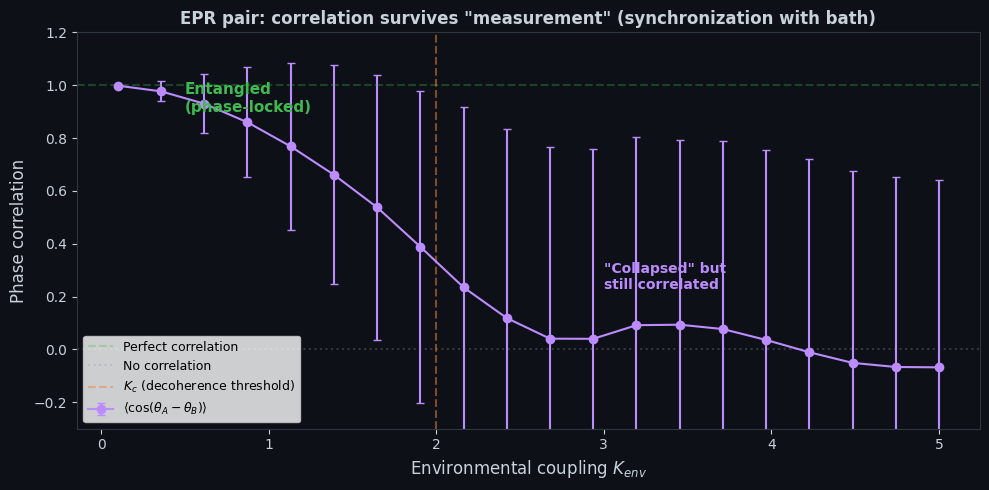
4.3 EPR: entanglement as pre-established synchronization#

Two particles that interacted are two oscillators that phase-locked through the shared medium. When they separate, they carry their phase relationship — not as a local hidden variable (Bell rules that out), but as a synchronization state of the medium itself.

The phase relationship isn’t a property of the particles. It is a property of the medium between them. The medium’s impedance at quantum scales preserves phase coherence across spatial separation — the “platform” connecting them hasn’t decohered.

Why EPR correlations aren’t “spooky”: you wouldn’t call it spooky if two metronomes on a swing, separated and placed on rigid tables, were later found ticking in phase. They synchronized before separation. Measuring one tells you about the other because they share phase history through the medium.

What Bell rules out is local classical hidden variables — values carried by the particles independently. But a synchronization state of the medium isn’t local to either particle. It is a property of the medium’s phase field. The medium is nonlocal in exactly the way QM requires, without requiring “action at a distance” — because it’s not action. It’s pre-established phase coherence that hasn’t yet been disrupted by coupling to a decoherent environment.

4.4 Connection to Non-Injectivity#

The Law of Genealogical Non-Injectivity states: at equilibrium, the measure over all paths to a given state is uniform. Once the system synchronizes with the detector, it doesn’t matter which path led to the measurement outcome. The synchronized state has multiple lineages. History is gauge. The detector click is ground truth.

def simulate_entangled_pair(K_env, K_c=2.0, N_trials=500, N_bath=50, dt=0.05, T=30.0):
    """Simulate two phase-locked oscillators coupling to independent baths.
    
    Returns the correlation between their phases after environmental coupling.
    
    K_env: coupling strength to environment (detector).
    When K_env > K_c, each oscillator synchronizes with its local bath
    ("measurement"), but mutual correlation is preserved because both
    started phase-locked.
    """
    rng = np.random.default_rng(123)
    correlations = []
    
    for _ in range(N_trials):
        # Two oscillators start perfectly phase-locked (entangled)
        theta_shared = rng.uniform(0, 2 * np.pi)
        theta_A = theta_shared
        theta_B = theta_shared  # same phase = entangled
        omega_A = 1.0
        omega_B = 1.0
        
        # Two independent baths (detectors)
        bath_A = rng.uniform(0, 2 * np.pi, N_bath)
        omega_bath_A = rng.standard_cauchy(N_bath) * 0.3
        bath_B = rng.uniform(0, 2 * np.pi, N_bath)
        omega_bath_B = rng.standard_cauchy(N_bath) * 0.3
        
        steps = int(T / dt)
        for _ in range(steps):
            # Bath A order parameter
            zA = np.mean(np.exp(1j * bath_A))
            rA, psiA = np.abs(zA), np.angle(zA)
            
            # Bath B order parameter  
            zB = np.mean(np.exp(1j * bath_B))
            rB, psiB = np.abs(zB), np.angle(zB)
            
            # Oscillator A couples to bath A
            dtheta_A = omega_A + K_env * rA * np.sin(psiA - theta_A)
            theta_A += dtheta_A * dt
            
            # Oscillator B couples to bath B
            dtheta_B = omega_B + K_env * rB * np.sin(psiB - theta_B)
            theta_B += dtheta_B * dt
            
            # Bath oscillators evolve (each coupled to its own mean field + the system oscillator)
            for i in range(N_bath):
                dbath_A = omega_bath_A[i] + K_env/N_bath * rA * np.sin(psiA - bath_A[i])
                bath_A[i] += dbath_A * dt
                dbath_B = omega_bath_B[i] + K_env/N_bath * rB * np.sin(psiB - bath_B[i])
                bath_B[i] += dbath_B * dt
        
        # Correlation: cos of phase difference (1 = perfectly correlated)
        correlations.append(np.cos(theta_A - theta_B))
    
    return np.mean(correlations), np.std(correlations)


# Scan environmental coupling
K_env_values = np.linspace(0.1, 5.0, 20)
corr_means = []
corr_stds = []

for K_env in K_env_values:
    mean, std = simulate_entangled_pair(K_env, N_trials=200)
    corr_means.append(mean)
    corr_stds.append(std)

corr_means = np.array(corr_means)
corr_stds = np.array(corr_stds)

fig, ax = plt.subplots(figsize=(10, 5))
ax.errorbar(K_env_values, corr_means, yerr=corr_stds, fmt='o-',
            color='#bc8cff', markersize=6, capsize=3, linewidth=1.5,
            label='$\\langle\\cos(\\theta_A - \\theta_B)\\rangle$')
ax.axhline(1.0, color='#3fb950', linestyle='--', alpha=0.3, label='Perfect correlation')
ax.axhline(0.0, color='#8b949e', linestyle=':', alpha=0.3, label='No correlation')
ax.axvline(2.0, color='#f0883e', linestyle='--', alpha=0.5, label='$K_c$ (decoherence threshold)')

ax.annotate('Entangled\n(phase-locked)', xy=(0.5, 0.9), fontsize=11,
            color='#3fb950', fontweight='bold')
ax.annotate('"Collapsed" but\nstill correlated', xy=(3.0, corr_means[14] + 0.15), fontsize=10,
            color='#bc8cff', fontweight='bold')

ax.set_xlabel('Environmental coupling $K_{env}$', fontsize=12)
ax.set_ylabel('Phase correlation', fontsize=12)
ax.set_title('EPR pair: correlation survives "measurement" (synchronization with bath)',
             fontsize=12, fontweight='bold')
ax.legend(loc='lower left', fontsize=9)
ax.set_facecolor('#0d1117')
fig.patch.set_facecolor('#0d1117')
ax.tick_params(colors='#c9d1d9')
ax.xaxis.label.set_color('#c9d1d9')
ax.yaxis.label.set_color('#c9d1d9')
ax.title.set_color('#c9d1d9')
for spine in ax.spines.values():
    spine.set_color('#30363d')
ax.set_ylim(-0.3, 1.2)
plt.tight_layout()
plt.show()

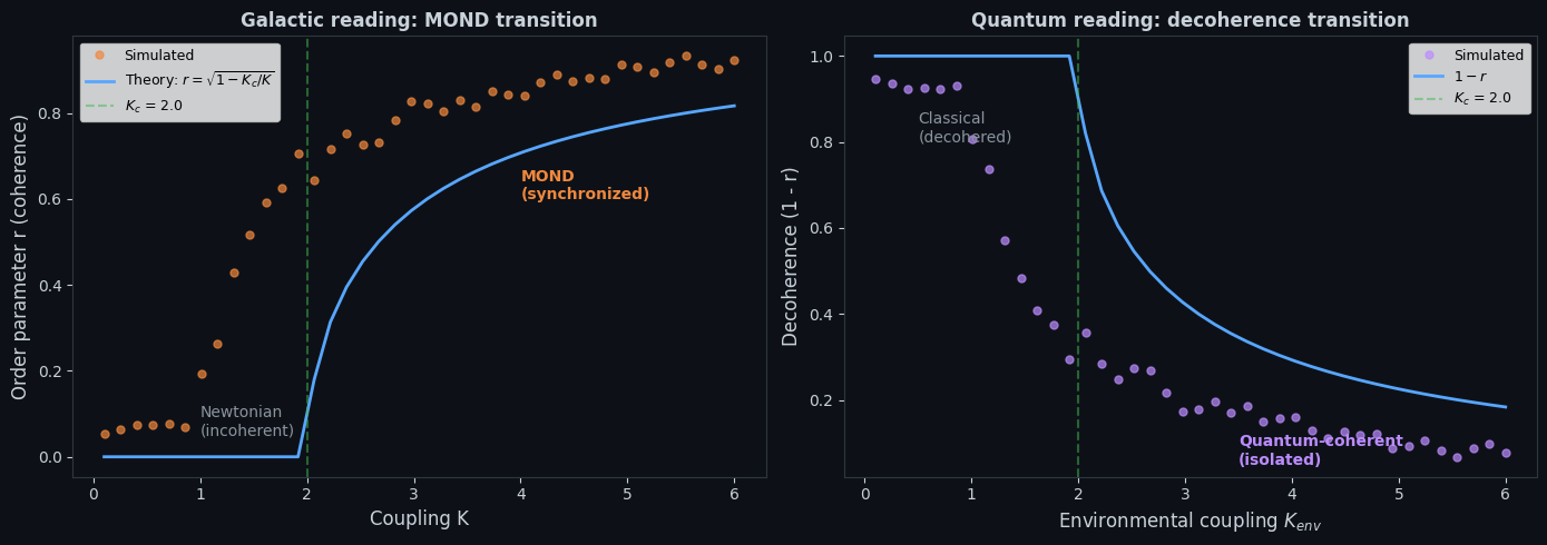
../_images/88c166b1f51ba2477df571ab486f22ad2b37424454a7823fecb8fbf4b56db6eb.png

5. Decoherence as Loss of Synchronization#

The quantum-to-classical transition is the Kuramoto transition on the viscous branch.

A quantum system isolated from its environment sits at the Stribeck minimum — low friction, weak coupling, phase coherence preserved. As environmental coupling increases (moving right on the curve), viscous drag rises. The environment provides too many incoherent oscillators. The system’s phase-locking with itself (superposition) is overwhelmed by phase-locking with the bath (decoherence).

“Collapse” is not destruction of information. It is the system synchronizing with a new, much larger set of oscillators. The superposition doesn’t vanish — it becomes a synchronization state shared across \(10^{23}\) detector atoms, where the phase information is irretrievable in practice but not in principle.

This is exactly the metronome picture: if you take a metronome off the swing and bolt it to a massive table (the detector), it doesn’t stop oscillating. It synchronizes with the table. The table is too heavy to move, so the metronome conforms to the table’s phase (which is effectively zero — classical rest). The metronome has “collapsed” into the table’s reference frame.

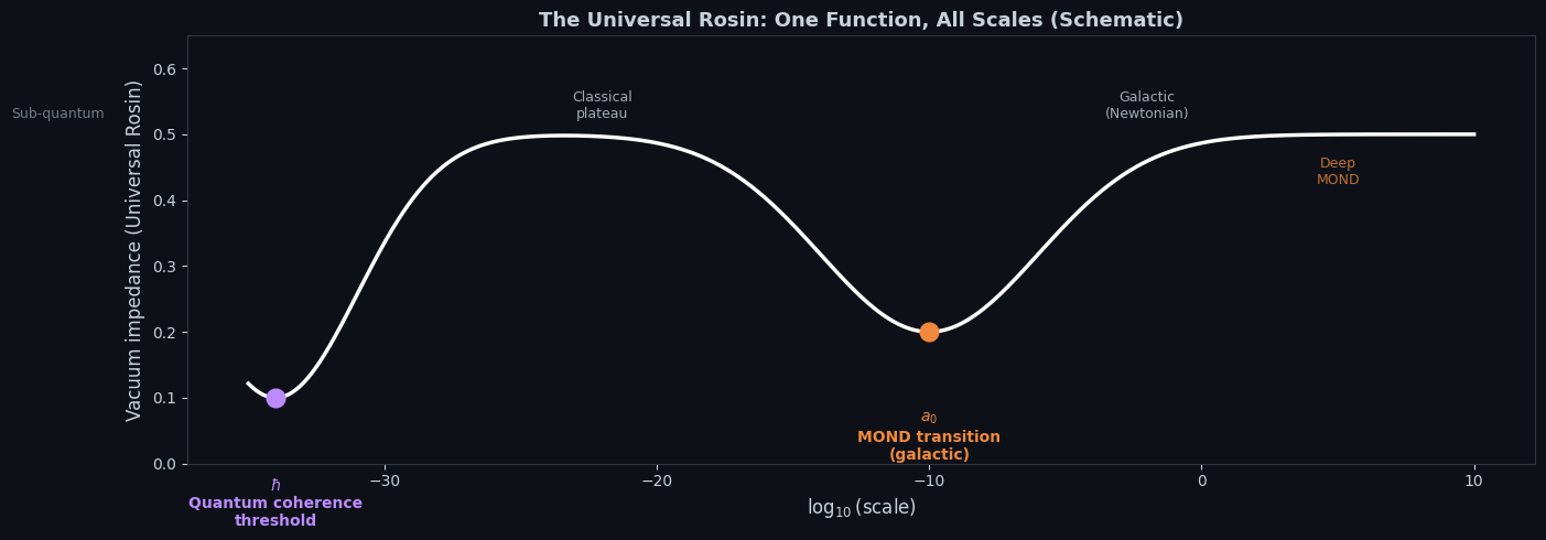
The \(\hbar\) connection#

\(\hbar\) is the unit of action — the unit of phase-space area. In the synchronization picture, \(\hbar\) sets the minimum phase-space volume where the medium can maintain coherent oscillation. Below this scale, the medium cannot support distinct phase relationships. Above it, phase coherence is possible but fragile — any coupling to a macroscopic bath that exceeds the Stribeck minimum will destroy it.

Just as \(a_0\) is the galactic impedance-matching point (where the medium transitions from stiff to compliant), \(\hbar\) is the quantum impedance-matching point (where the medium transitions from supporting coherent phase to not supporting it).

The Universal Rosin, then, is not a single number but a function with at least two critical points:

Critical point	Scale	Physical meaning
\(\hbar\)	Quantum	Minimum phase-space area for coherent oscillation
\(a_0\)	Galactic	Acceleration at which collective synchronization activates
\(\Lambda\)?	Cosmological	Impedance of the vacuum at the largest scales

These may all be aspects of the same curve — the vacuum’s Stribeck function evaluated at different scales.

# Schematic: the Universal Rosin across all scales
# This is conceptual — showing how one impedance function
# might connect quantum, classical, and galactic regimes.

log_scale = np.linspace(-35, 10, 1000)  # log10 of coupling/scale

# Construct a schematic multi-branch Stribeck curve
# Two minima: one at quantum scale, one at galactic scale
def schematic_rosin(x):
    """Schematic Universal Rosin with quantum and galactic branches."""
    # Quantum minimum near hbar scale (~-34)
    quantum_well = 0.4 * np.exp(-0.5 * ((x + 34) / 3) ** 2)
    # Galactic minimum near a0 scale (~-10)  
    galactic_well = 0.3 * np.exp(-0.5 * ((x + 10) / 4) ** 2)
    # Baseline impedance
    baseline = 0.5
    return baseline - quantum_well - galactic_well

impedance = schematic_rosin(log_scale)

fig, ax = plt.subplots(figsize=(14, 5))
ax.plot(log_scale, impedance, 'w-', linewidth=2.5)

# Mark the critical points
for x_pos, label, color in [
    (-34, '$\\hbar$\nQuantum coherence\nthreshold', '#bc8cff'),
    (-10, '$a_0$\nMOND transition\n(galactic)', '#f0883e'),
]:
    y_pos = schematic_rosin(x_pos)
    ax.plot(x_pos, y_pos, 'o', color=color, markersize=12, zorder=5)
    ax.annotate(label, xy=(x_pos, y_pos), xytext=(x_pos, y_pos - 0.12),
                fontsize=10, color=color, fontweight='bold',
                ha='center', va='top')

# Mark regimes
regime_labels = [
    (-42, 0.52, 'Sub-quantum', '#8b949e'),
    (-22, 0.52, 'Classical\nplateau', '#c9d1d9'),
    (-2, 0.52, 'Galactic\n(Newtonian)', '#c9d1d9'),
    (5, 0.42, 'Deep\nMOND', '#f0883e'),
]
for x, y, label, color in regime_labels:
    ax.text(x, y, label, fontsize=9, color=color, ha='center', va='bottom', alpha=0.8)

ax.set_xlabel('$\\log_{10}$(scale)', fontsize=12)
ax.set_ylabel('Vacuum impedance (Universal Rosin)', fontsize=12)
ax.set_title('The Universal Rosin: One Function, All Scales (Schematic)', fontsize=13, fontweight='bold')
ax.set_facecolor('#0d1117')
fig.patch.set_facecolor('#0d1117')
ax.tick_params(colors='#c9d1d9')
ax.xaxis.label.set_color('#c9d1d9')
ax.yaxis.label.set_color('#c9d1d9')
ax.title.set_color('#c9d1d9')
for spine in ax.spines.values():
    spine.set_color('#30363d')
ax.set_ylim(0, 0.65)
plt.tight_layout()
plt.show()

../_images/c3c9533f0ae4d31128e4f43bc1c40ea6da86980cc46f2361c3d6aab9bc77abcc.png

6. Summary: What the Quantum Branch Resolves#

Open question	Standard answer	Synchronization answer
What is “measurement”?	Undefined (Copenhagen)	Synchronization with detector: \(K_{\text{eff}} > K_c\)
When does collapse happen?	When “observed” (circular)	When system-apparatus coupling exceeds impedance threshold
Why are EPR correlations nonlocal?	“Spooky action at a distance”	Pre-established phase coherence in the medium; not action, not local
What is decoherence?	Loss of off-diagonal density matrix elements	Loss of synchronization: viscous branch of Stribeck curve
What sets the quantum/classical boundary?	Unspecified	The Stribeck minimum: impedance-matching point between coherent and viscous regimes
Is \(\hbar\) a fundamental constant or derived?	Fundamental	Impedance-matching point of the vacuum Stribeck curve at quantum scales (parallel to \(a_0\) at galactic scales)

The measurement problem is a solved problem in disguise. It is the same phase transition as the MOND transition, read on the opposite branch of the Universal Rosin.

What remains#

Quantitative decoherence rates. Can the Stribeck-Kuramoto model reproduce measured decoherence timescales for specific systems (superconducting qubits, photon polarization, etc.)?
Bell inequality. The framework must reproduce Bell violation at the same quantitative level as standard QM. The medium’s nonlocality (phase-field coherence across spatial separation) must produce the correct \(2\sqrt{2}\) Tsirelson bound.
The Stribeck minimum. Is there a measurable physical quantity that corresponds to the impedance minimum between quantum and classical regimes? Candidate: the decoherence rate as a function of environmental coupling, measured across the quantum-to-classical transition.

License: CC0 — No rights reserved.