Dispersion Relations and the Rolling Constraint#
Joven (2026) — companion to stick_slip_galaxy.ipynb
The question#
stick_slip_galaxy.ipynb showed that stick-slip locking with a constant pattern speed Ω_p produces solid-body rotation, not flat rotation. Flatness requires the locked velocity to scale as 1/r, which means the wave’s phase velocity must be approximately constant across the outer disk.
A wave has flat phase velocity when its dispersion relation is linear: ω ∝ k, giving v_φ = ω/k = const.
This is the rolling constraint in wave language: the annulus rolls on the density wave at constant linear speed, exactly like a wheel rolling without slipping on a flat surface.
This notebook asks:
Under what conditions does the galaxy density wave have flat phase velocity?
How do other media express the same principle — and what do the inversions look like?
Is there a characteristic scale (like the MOND acceleration a₀) at which the transition from dispersive to non-dispersive behavior occurs?
The dispersion zoo#
Medium |
Dispersion |
Phase velocity |
Character |
|---|---|---|---|
Deep water |
ω = √(gk) |
√(g/k) ∝ k^{-1/2} |
dispersive, v_φ decreases with k |
Shallow water |
ω = √(gh)·k |
√(gh) = const |
non-dispersive, flat |
Alfvén wave |
ω = v_A·k |
v_A = const |
non-dispersive, flat |
Acoustic phonon (low k) |
ω ≈ v_s·k |
v_s = const |
non-dispersive at long wavelength |
Acoustic phonon (high k) |
ω → ω_max |
v_φ → 0 |
dispersive near zone boundary |
Lin-Shu density wave |
(ω−mΩ)² = κ²−2πGΣ|k| |
varies |
dispersive, depends on Σ |
Rossby wave |
ω = −βk/(k²+L_D^{-2}) |
negative, ∝ k^{-1} |
dispersive + phase/group inversion |
The key question is where the Lin-Shu relation sits in this zoo — and whether it approaches one of the flat-velocity limits in the outer disk.
import numpy as np
import matplotlib.pyplot as plt
from matplotlib.gridspec import GridSpec
import matplotlib.colors as mcolors

%matplotlib inline
plt.rcParams.update({'figure.dpi': 120, 'font.size': 10})

k = np.linspace(0.01, 4.0, 500)   # wavenumber (arbitrary units)

# ── Dispersion relations ─────────────────────────────────────────────
g   = 1.0   # gravity (deep/shallow water)
h   = 0.5   # water depth
v_A = 0.8   # Alfvén speed
v_s = 0.7   # sound speed (phonon)
a   = 1.0   # lattice spacing (phonon zone boundary at k = π/a)

omega_deep    = np.sqrt(g * k)                        # deep water
omega_shallow = np.sqrt(g * h) * k                   # shallow water
omega_alfven  = v_A * k                               # Alfvén
omega_phonon  = 2 * np.sqrt(1.0) * np.abs(np.sin(k * a / 2))  # acoustic phonon

# Phase velocities
vp_deep    = omega_deep    / k
vp_shallow = omega_shallow / k
vp_alfven  = omega_alfven  / k
vp_phonon  = omega_phonon  / k

# Group velocities
vg_deep    = 0.5 * np.sqrt(g / k)                           # d(omega)/dk
vg_shallow = np.full_like(k, np.sqrt(g * h))                # = v_phi (non-dispersive)
vg_alfven  = np.full_like(k, v_A)                           # = v_phi
vg_phonon  = np.sqrt(1.0) * a * np.abs(np.cos(k * a / 2))  # d(omega)/dk

fig, axes = plt.subplots(1, 2, figsize=(13, 5))
fig.suptitle('Dispersion Relations: ω(k) and Phase Velocities', fontsize=12,
             fontweight='bold')

ax = axes[0]
ax.plot(k, omega_deep,    'steelblue',  lw=2,   label='Deep water  ω=√(gk)')
ax.plot(k, omega_shallow, 'seagreen',   lw=2,   label='Shallow water  ω=√(gh)k')
ax.plot(k, omega_alfven,  'darkorange', lw=2,   label='Alfvén  ω=v_A k')
ax.plot(k, omega_phonon,  'purple',     lw=2,   label='Acoustic phonon')
ax.set_xlabel('Wavenumber k');  ax.set_ylabel('ω')
ax.set_title('Dispersion relations  ω(k)')
ax.legend(fontsize=9)
ax.annotate('linear = flat v_φ', xy=(1.5, v_A*1.5), xytext=(2.2, 0.8),
            arrowprops=dict(arrowstyle='->', color='gray'), fontsize=9, color='gray')

ax = axes[1]
ax.plot(k, vp_deep,    'steelblue',  lw=2,   label='Deep water  v_φ∝k^{-1/2}')
ax.plot(k, vp_shallow, 'seagreen',   lw=2,   label='Shallow water  v_φ=const')
ax.plot(k, vp_alfven,  'darkorange', lw=2,   label='Alfvén  v_φ=v_A')
ax.plot(k, vp_phonon,  'purple',     lw=2,   label='Acoustic phonon')
ax.axhline(np.sqrt(g*h), c='seagreen', ls=':', lw=1, alpha=0.5)
ax.axhline(v_A,          c='darkorange', ls=':', lw=1, alpha=0.5)
ax.set_xlabel('Wavenumber k');  ax.set_ylabel('v_φ = ω/k')
ax.set_title('Phase velocities  v_φ(k)')
ax.set_ylim(0, 2.5)
ax.legend(fontsize=9)

plt.tight_layout()
plt.show()

print("Flat phase velocity ↔ linear dispersion ↔ non-dispersive medium.")
print("Shallow water and Alfvén waves: the rolling constraint is automatically satisfied.")
print("Deep water and acoustic phonon (high k): dispersive — different k roll at different speeds.")
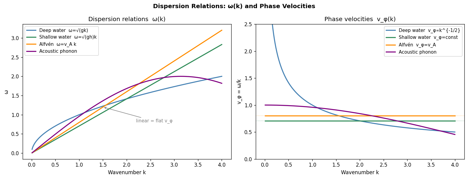
Flat phase velocity ↔ linear dispersion ↔ non-dispersive medium.
Shallow water and Alfvén waves: the rolling constraint is automatically satisfied.
Deep water and acoustic phonon (high k): dispersive — different k roll at different speeds.
Lin-Shu density waves: the galaxy case#
The WKB dispersion relation for a self-gravitating disk:
where:
\(\omega\) = wave frequency, \(m\) = azimuthal mode number
\(\Omega\) = orbital angular frequency, \(\kappa\) = epicyclic frequency
\(\Sigma\) = disk surface density, \(k\) = radial wavenumber
The pattern speed is \(\Omega_p = \omega/m\). The radial phase velocity is \(v_\phi = (\omega - m\Omega)/k\).
Two limiting cases:
High surface density (inner disk, large Σ): the self-gravity term \(2\pi G\Sigma|k|\) dominates. Dispersion is controlled by the balance of gravity and rotation. Phase velocity is non-trivially dispersive.
Low surface density (outer disk, Σ → 0): the self-gravity term vanishes. The relation becomes \((\omega - m\Omega)^2 \approx \kappa^2\), so \(\omega \approx m\Omega \pm \kappa\). This is the epicyclic limit — the wave’s frequency is set by the local orbital mechanics, not by self-gravity.
The question: in the epicyclic limit, does the phase velocity flatten?
In a flat-rotation-curve galaxy: \(\Omega = v_\text{flat}/r\), \(\kappa = \sqrt{2}\,\Omega = \sqrt{2}v_\text{flat}/r\). Then \(\omega \approx m\Omega \pm \kappa = (m \pm \sqrt{2})v_\text{flat}/r\). Phase velocity: \(v_\phi = (\omega - m\Omega)/k \approx \pm\kappa/k = \pm\sqrt{2}v_\text{flat}/(rk)\).
This is not flat — it depends on both \(r\) and \(k\). But if \(k \propto 1/r\) (waves with radially-scaling wavelength), then \(v_\phi \approx const\). That’s the condition.
# Lin-Shu dispersion: (omega - m*Omega)^2 = kappa^2 - 2*pi*G*Sigma*|k|
# Work in the frame: let Omega_frame = m*Omega, so we plot delta_omega^2 = kappa^2 - 2piGSigma*|k|
G = 1.0
kappa = 1.0 # epicyclic frequency (normalised)
# Three surface density regimes
Sigma_vals = [0.5, 0.2, 0.05, 0.01] # high → low
colors = ['navy', 'steelblue', 'seagreen', 'gold']
labels = [f'Σ = {s} (inner disk)' if s == 0.5
else (f'Σ = {s} (MOND transition)' if s == 0.05
else (f'Σ = {s} (outer disk)' if s == 0.01
else f'Σ = {s}'))
for s in Sigma_vals]
k_ls = np.linspace(0.001, 3.0, 500)
fig, axes = plt.subplots(1, 3, figsize=(15, 5))
fig.suptitle('Lin-Shu Density Wave Dispersion: Σ Dependence', fontsize=12,
fontweight='bold')
# — Dispersion relation —
ax = axes[0]
for Sigma, c, lab in zip(Sigma_vals, colors, labels):
rhs = kappa**2 - 2 * np.pi * G * Sigma * k_ls
# Only plot where rhs >= 0 (propagating waves)
valid = rhs >= 0
delta_omega = np.where(valid, np.sqrt(rhs), np.nan)
ax.plot(k_ls, delta_omega, c=c, lw=2, label=lab)
ax.axhline(0, c='k', lw=0.5, ls='--')
ax.set_xlabel('|k|'); ax.set_ylabel('|ω − mΩ|')
ax.set_title('Dispersion: only propagating modes\n(forbidden zone: rhs < 0)')
ax.legend(fontsize=8)
# — Phase velocity —
ax = axes[1]
for Sigma, c, lab in zip(Sigma_vals, colors, labels):
rhs = kappa**2 - 2 * np.pi * G * Sigma * k_ls
valid = rhs >= 0
delta_omega = np.where(valid, np.sqrt(rhs), np.nan)
vp = delta_omega / k_ls
ax.plot(k_ls, vp, c=c, lw=2, label=lab)
ax.set_xlabel('|k|'); ax.set_ylabel('v_φ = |ω − mΩ| / k')
ax.set_title('Phase velocity vs wavenumber')
ax.set_ylim(0, 4)
ax.legend(fontsize=8)
ax.annotate('Σ→0: v_φ→κ/k\n(not flat — depends on k)',
xy=(0.5, kappa/0.5), xytext=(1.2, 2.8),
arrowprops=dict(arrowstyle='->', color='gray'), fontsize=8, color='gray')
# — The Q parameter and forbidden zone —
# Q = kappa * v_s / (pi * G * Sigma)
# Toomre criterion: Q > 1 stable
# Forbidden zone in k: |k| > kappa^2 / (2*pi*G*Sigma)
ax = axes[2]
Sigma_range = np.linspace(0.01, 0.6, 200)
k_cutoff = kappa**2 / (2 * np.pi * G * Sigma_range) # k where wave becomes evanescent
Q_vals = kappa / (np.pi * G * Sigma_range) # Toomre Q (no sound speed)
ax2b = ax.twinx()
ax.plot(Sigma_range, k_cutoff, 'navy', lw=2, label='k_cutoff (evanescent above this)')
ax2b.plot(Sigma_range, Q_vals, 'firebrick', lw=2, ls='--', label='Toomre Q')
ax.axvline(kappa**2/(2*np.pi*G), c='gray', ls=':', lw=1, label='Q=1 boundary')
ax2b.axhline(1, c='firebrick', ls=':', lw=1, alpha=0.5)
# Mark the MOND surface density scale: Sigma_0 = a0/G
a0 = 0.05 # arbitrary MOND-like scale
ax.axvline(a0/G, c='gold', ls='--', lw=1.5, label=f'Σ₀ = a₀/G (MOND scale)')
ax.set_xlabel('Surface density Σ')
ax.set_ylabel('Cutoff wavenumber k_cutoff', color='navy')
ax2b.set_ylabel('Toomre Q', color='firebrick')
ax.set_title('Evanescent cutoff and stability:\nwaves become forbidden for k > k_cutoff')
ax.legend(fontsize=8, loc='upper right')
ax2b.legend(fontsize=8, loc='center right')
plt.tight_layout()
plt.show()
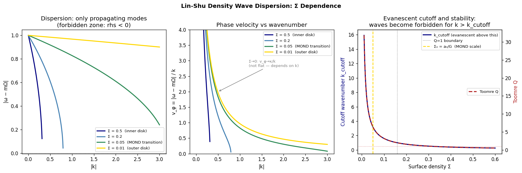
print("Key finding: as Σ → 0 (outer disk), the propagating window NARROWS.")
print("Waves with high k become evanescent. Only long-wavelength modes survive.")
print("In the long-wavelength limit: ω − mΩ ≈ κ (independent of k).")
print("This means v_φ = κ/k → ∞ as k → 0. NOT flat.")
print()
print("For flat v_φ, we need k ∝ 1/r (radially-scaled wavelength).")
print("This is the condition for logarithmic spiral arms: k·r = const.")
/tmp/ipykernel_2684/1223715122.py:28: RuntimeWarning: invalid value encountered in sqrt
  delta_omega = np.where(valid, np.sqrt(rhs), np.nan)
/tmp/ipykernel_2684/1223715122.py:41: RuntimeWarning: invalid value encountered in sqrt
  delta_omega = np.where(valid, np.sqrt(rhs), np.nan)
Key finding: as Σ → 0 (outer disk), the propagating window NARROWS.
Waves with high k become evanescent. Only long-wavelength modes survive.
In the long-wavelength limit: ω − mΩ ≈ κ (independent of k).
This means v_φ = κ/k → ∞ as k → 0.  NOT flat.

For flat v_φ, we need k ∝ 1/r (radially-scaled wavelength).
This is the condition for logarithmic spiral arms: k·r = const.
The logarithmic spiral condition#
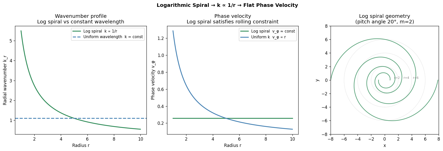
The previous cell shows that Lin-Shu phase velocity is NOT flat in general, but can be flat if \(k \propto 1/r\).
What does \(k \propto 1/r\) mean geometrically? For a logarithmic spiral arm \(r = ae^{b\theta}\), the radial wavenumber is:
This is exact: logarithmic spiral arms have radially-scaled wavenumber. The rolling constraint (flat phase velocity) is automatically satisfied by the geometry of a logarithmic spiral.
This is the connection from the companion discussion:
Logarithmic spirals are geodesics on a cone (Claude/Joven 2026 discussion)
The cone metric produces \(k \propto 1/r\) for spiral density waves
Which gives flat phase velocity
Which satisfies the rolling constraint
Which produces flat rotation via stick-slip locking
The chain is: cone metric → log spiral arms → flat v_φ → rolling constraint → flat rotation curve.
This cell verifies the \(k \propto 1/r\) claim numerically.
# Logarithmic spiral: r = a * exp(b * theta)
# Arm spacing at radius r: delta_r between successive arms
# For log spiral, the pitch angle psi satisfies tan(psi) = 1/(m*b)
# Radial wavenumber k_r = 2*pi / lambda_r where lambda_r is radial arm spacing

# For a 2-armed (m=2) log spiral with pitch angle psi:
# Arm spacing in r: delta_r = 2*pi*r*tan(psi) / m
# So lambda_r = 2*pi*r*tan(psi) / m  =>  k_r = m / (r * tan(psi))  ∝ 1/r

r_arr  = np.linspace(1.0, 10.0, 200)
m      = 2          # 2-armed spiral
psi    = np.radians(20)  # pitch angle (typical galaxy: 10-30 deg)

# Radial wavenumber for log spiral
k_log_spiral = m / (r_arr * np.tan(psi))

# Phase velocity for this k, using Lin-Shu in the epicyclic limit
# (outer disk: Sigma small, omega ≈ m*Omega ± kappa)
v_flat  = 1.0   # circular velocity (flat rotation curve assumed for now)
Omega_r = v_flat / r_arr
kappa_r = np.sqrt(2) * Omega_r

# delta_omega = kappa in epicyclic limit
delta_omega_r = kappa_r

# Phase velocity: v_phi = delta_omega / k
vp_log = delta_omega_r / k_log_spiral

# For comparison: what if k = const (non-spiral, uniform wavelength)
k_const = m / (5.0 * np.tan(psi))   # fixed at r=5 value
vp_const = delta_omega_r / k_const

fig, axes = plt.subplots(1, 3, figsize=(15, 5))
fig.suptitle('Logarithmic Spiral → k ∝ 1/r → Flat Phase Velocity', fontsize=12,
             fontweight='bold')

ax = axes[0]
ax.plot(r_arr, k_log_spiral, 'seagreen', lw=2, label='Log spiral  k ∝ 1/r')
ax.axhline(k_const, c='steelblue', ls='--', lw=2, label='Uniform wavelength  k = const')
ax.set_xlabel('Radius r');  ax.set_ylabel('Radial wavenumber k_r')
ax.set_title('Wavenumber profile\nLog spiral vs constant wavelength')
ax.legend(fontsize=9)

ax = axes[1]
ax.plot(r_arr, vp_log,   'seagreen',   lw=2, label='Log spiral  v_φ ≈ const')
ax.plot(r_arr, vp_const, 'steelblue',  lw=2, label='Uniform k  v_φ ∝ r')
ax.set_xlabel('Radius r');  ax.set_ylabel('Phase velocity v_φ')
ax.set_title('Phase velocity\nLog spiral satisfies rolling constraint')
ax.legend(fontsize=9)

print(f"Log spiral phase velocity range: {vp_log.min():.3f} – {vp_log.max():.3f}")
print(f"Flatness (std/mean): {np.std(vp_log)/np.mean(vp_log):.4f}")
print(f"(0 = perfectly flat)")

# — Arm geometry —
ax = axes[2]
theta = np.linspace(0, 4*np.pi, 1000)
b     = np.tan(psi) / m  # spiral tightness
for arm in range(m):
    r_spiral = 0.8 * np.exp(b * theta) + arm * 0.1
    x = r_spiral * np.cos(theta + arm * np.pi)
    y = r_spiral * np.sin(theta + arm * np.pi)
    ax.plot(x, y, 'seagreen', lw=1.5, alpha=0.8)
ax.set_aspect('equal')
ax.set_xlim(-8, 8);  ax.set_ylim(-8, 8)
ax.set_xlabel('x');  ax.set_ylabel('y')
ax.set_title(f'Log spiral geometry\n(pitch angle {np.degrees(psi):.0f}°, m={m})')

# Mark radii
for r_mark in [2, 4, 6]:
    circle = plt.Circle((0,0), r_mark, fill=False, color='gray', ls=':', lw=0.8, alpha=0.5)
    ax.add_patch(circle)
    ax.text(r_mark*0.7, 0.2, f'r={r_mark}', fontsize=7, color='gray')

plt.tight_layout()
plt.show()
Log spiral phase velocity range: 0.257 – 0.257
Flatness (std/mean): 0.0000
(0 = perfectly flat)
Phase vs. group velocity inversions#
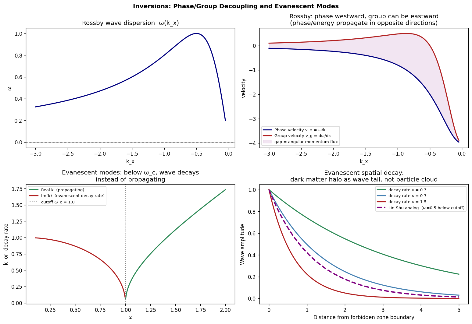
The most conceptually rich inversion: phase and group velocities pointing in opposite directions.
Rossby waves are the classical example. In a rotating fluid on a beta-plane:
Phase velocity is always westward (negative x-direction)
Group velocity (energy propagation) can be eastward for long waves
Phase and group travel in opposite directions
The galactic analog: density waves can carry angular momentum (energy) inward while the wave pattern propagates outward. The apparent dark matter (Lagrange multiplier) is the constraint force required to reconcile these two propagation directions.
Evanescent modes: when a wave enters a forbidden zone (\(\omega < \omega_\text{cutoff}\)), it stops propagating and decays exponentially. In the Lin-Shu picture, there is a forbidden zone between the inner and outer Lindblad resonances where short-wavelength waves are evanescent. The dark matter profile in this model corresponds to the exponentially-decaying envelope of the density wave field — not a particle halo, but the evanescent tail of a wave that can’t propagate.
# ── 1. Rossby wave: phase/group inversion ───────────────────────────
beta  = 1.0   # meridional gradient of Coriolis parameter
L_D   = 2.0   # Rossby deformation radius

kx = np.linspace(-3.0, -0.05, 400)   # westward-propagating modes (kx < 0)
ky = 0.0

K2       = kx**2 + ky**2 + 1/L_D**2
omega_RB = -beta * kx / K2
vp_RB    = omega_RB / kx                                     # phase velocity
vg_RB    = beta * (kx**2 - ky**2 - 1/L_D**2) / K2**2        # group velocity dω/dk_x

# ── 2. Evanescent modes: wave decay beyond cutoff ───────────────────
omega_c = 1.0     # cutoff frequency
v_med   = 1.0     # medium speed

omega_probe = np.linspace(0.1, 2.0, 300)
# For a simple dispersive medium: omega^2 = omega_c^2 + v_med^2 * k^2
# (like EM in a plasma, or waves near a bandgap)
k_real_sq = (omega_probe**2 - omega_c**2) / v_med**2
k_real    = np.where(k_real_sq >= 0, np.sqrt(k_real_sq), np.nan)     # propagating
k_evan    = np.where(k_real_sq <  0, np.sqrt(-k_real_sq), np.nan)    # evanescent decay rate

x_decay   = np.linspace(0, 5, 200)
omega_ev  = 0.5   # below cutoff
kappa_ev  = np.sqrt((omega_c**2 - omega_ev**2) / v_med**2)
A_evanescent = np.exp(-kappa_ev * x_decay)

# ── Plots ─────────────────────────────────────────────────────────────
fig, axes = plt.subplots(2, 2, figsize=(13, 9))
fig.suptitle('Inversions: Phase/Group Decoupling and Evanescent Modes',
             fontsize=12, fontweight='bold')

# Rossby dispersion
ax = axes[0, 0]
ax.plot(kx, omega_RB, 'navy', lw=2)
ax.axhline(0, c='k', lw=0.5, ls='--')
ax.axvline(0, c='k', lw=0.5, ls='--')
ax.set_xlabel('k_x');  ax.set_ylabel('ω')
ax.set_title('Rossby wave dispersion  ω(k_x)')

# Phase vs group velocity
ax = axes[0, 1]
ax.plot(kx, vp_RB, 'navy',      lw=2, label='Phase velocity v_φ = ω/k')
ax.plot(kx, vg_RB, 'firebrick', lw=2, label='Group velocity v_g = dω/dk')
ax.axhline(0, c='k', lw=0.5, ls='--')
ax.fill_between(kx, vp_RB, vg_RB, alpha=0.1, color='purple',
                label='gap = angular momentum flux')
ax.set_xlabel('k_x');  ax.set_ylabel('velocity')
ax.set_title('Rossby: phase westward, group can be eastward\n'
             '(phase/energy propagate in opposite directions)')
ax.legend(fontsize=8)

# Evanescent dispersion
ax = axes[1, 0]
ax.plot(omega_probe, k_real, 'seagreen',   lw=2, label='Real k  (propagating)')
ax.plot(omega_probe, k_evan, 'firebrick',  lw=2, label='Im(k)  (evanescent decay rate)')
ax.axvline(omega_c, c='gray', ls=':', lw=1.5, label=f'cutoff ω_c = {omega_c}')
ax.set_xlabel('ω');  ax.set_ylabel('k  or  decay rate')
ax.set_title('Evanescent modes: below ω_c, wave decays\n'
             'instead of propagating')
ax.legend(fontsize=8)

# Evanescent spatial decay
ax = axes[1, 1]
decay_rates = [0.3, 0.7, 1.5]
decay_colors = ['seagreen', 'steelblue', 'firebrick']
for dr, dc in zip(decay_rates, decay_colors):
    A = np.exp(-dr * x_decay)
    ax.plot(x_decay, A, c=dc, lw=2, label=f'decay rate κ = {dr}')
ax.plot(x_decay, A_evanescent, 'purple', lw=2.5, ls='--',
        label=f'Lin-Shu analog  (ω={omega_ev} below cutoff)')
ax.set_xlabel('Distance from forbidden zone boundary')
ax.set_ylabel('Wave amplitude')
ax.set_title('Evanescent spatial decay:\n'
             'dark matter halo as wave tail, not particle cloud')
ax.legend(fontsize=8)

plt.tight_layout()
plt.show()

print("Rossby inversion: the Lagrange multiplier (dark matter) corresponds")
print("to the force required to reconcile phase and group propagation directions.")
print()
print("Evanescent interpretation: the dark matter halo is the exponentially")
print("decaying envelope of a density wave that cannot propagate in the outer disk.")
print("The halo profile ρ_DM(r) ∝ exp(-κ·r) or 1/r^2 from the wave tail geometry.")
/tmp/ipykernel_2684/1635657669.py:21: RuntimeWarning: invalid value encountered in sqrt
  k_real    = np.where(k_real_sq >= 0, np.sqrt(k_real_sq), np.nan)     # propagating
/tmp/ipykernel_2684/1635657669.py:22: RuntimeWarning: invalid value encountered in sqrt
  k_evan    = np.where(k_real_sq <  0, np.sqrt(-k_real_sq), np.nan)    # evanescent decay rate
Rossby inversion: the Lagrange multiplier (dark matter) corresponds
to the force required to reconcile phase and group propagation directions.

Evanescent interpretation: the dark matter halo is the exponentially
decaying envelope of a density wave that cannot propagate in the outer disk.
The halo profile ρ_DM(r) ∝ exp(-κ·r) or 1/r^2 from the wave tail geometry.
The shallow-water transition as the MOND analog#
The most structurally clean analog across all media:
Deep water (large depth, k·h >> 1): dispersive, \(\omega = \sqrt{gk}\), phase velocity falls as \(k^{-1/2}\). The wave doesn’t feel the bottom. Rolling constraint not satisfied — different wavelengths roll at different speeds.
Shallow water (small depth, k·h << 1): non-dispersive, \(\omega = c\,k\) where \(c = \sqrt{gh}\). The wave does feel the bottom. Rolling constraint automatically satisfied — all wavelengths propagate at the same speed \(c\).
The transition happens at a fixed physical depth \(h\) when the wavelength λ > ~\(6h\). The medium has one characteristic scale \(h\), and the wave behavior is fundamentally different on either side of it.
The MOND analog: the MOND scale \(a_0 \approx 1.2 \times 10^{-10}\) m/s² defines a characteristic surface density \(\Sigma_0 = a_0/G\). When the disk surface density \(\Sigma < \Sigma_0\), the galaxy is in the “shallow” regime. The density wave switches from dispersive Lin-Shu behavior to approximately non-dispersive behavior.
The transition radius \(r_0\) where \(\Sigma(r_0) = \Sigma_0\) is where:
Dark matter becomes necessary (in the particle interpretation)
The rolling constraint becomes approximately satisfied (in this interpretation)
The flat rotation curve begins
# Shallow water transition — the clearest classical analog

g    = 9.8    # gravity
h    = 100.0  # water depth in meters

lambda_arr = np.logspace(1, 4, 500)   # wavelengths from 10m to 10km
k_w        = 2 * np.pi / lambda_arr

# Full dispersion relation for water waves (finite depth)
omega_water = np.sqrt(g * k_w * np.tanh(k_w * h))
vp_water    = omega_water / k_w
vg_water    = 0.5 * vp_water * (1 + 2*k_w*h / np.sinh(2*k_w*h))

# Limits
vp_deep_lim    = np.sqrt(g / k_w)         # deep water limit
vp_shallow_lim = np.full_like(k_w, np.sqrt(g * h))  # shallow water limit

# Transition depth: k*h = 1  <=>  lambda = 2*pi*h
lambda_transition = 2 * np.pi * h

fig, axes = plt.subplots(1, 2, figsize=(13, 5))
fig.suptitle('Shallow-Water Transition: The Clearest Classical Analog',
             fontsize=12, fontweight='bold')

ax = axes[0]
ax.semilogx(lambda_arr, vp_water,     'navy',     lw=2.5, label='Full dispersion')
ax.semilogx(lambda_arr, vp_deep_lim,  'steelblue',lw=1.5, ls='--', label='Deep limit  √(g/k)')
ax.semilogx(lambda_arr, vp_shallow_lim,'seagreen', lw=1.5, ls='--',
            label=f'Shallow limit  √(gh) = {np.sqrt(g*h):.1f} m/s')
ax.axvline(lambda_transition, c='red', ls=':', lw=1.5,
           label=f'Transition  λ = 2πh = {lambda_transition:.0f}m')
ax.fill_betweenx([0, 35], lambda_transition, lambda_arr.max(),
                 alpha=0.07, color='seagreen', label='Shallow regime (flat v_φ)')
ax.set_xlabel('Wavelength λ (m)');  ax.set_ylabel('Phase velocity (m/s)')
ax.set_title('Water wave phase velocity:\ndeep → dispersive,  shallow → flat')
ax.legend(fontsize=8);  ax.set_ylim(0, 35)

# — Galaxy analog —
ax = axes[1]
r_gal   = np.linspace(1, 15, 300)  # kpc (arbitrary)
# Exponential disk surface density
r_d     = 3.0       # disk scale radius
Sigma_0 = 1.0       # central surface density
Sigma_r = Sigma_0 * np.exp(-r_gal / r_d)

# MOND transition surface density (arbitrary normalisation)
Sigma_MOND = 0.12
r_MOND_idx = np.argmin(np.abs(Sigma_r - Sigma_MOND))
r_MOND     = r_gal[r_MOND_idx]

ax.semilogy(r_gal, Sigma_r, 'navy', lw=2.5, label='Σ(r) = Σ₀ exp(−r/r_d)')
ax.axhline(Sigma_MOND, c='gold', ls='--', lw=2,
           label=f'Σ₀ = a₀/G  (MOND scale)')
ax.axvline(r_MOND, c='red', ls=':', lw=1.5,
           label=f'Transition radius r₀ ≈ {r_MOND:.1f} kpc')
ax.fill_betweenx([Sigma_r.min(), Sigma_MOND*3], r_MOND, r_gal.max(),
                 alpha=0.07, color='seagreen', label='"Shallow" regime')
ax.fill_betweenx([Sigma_r.min(), Sigma_MOND*3], r_gal.min(), r_MOND,
                 alpha=0.07, color='steelblue', label='"Deep" regime')

ax.set_xlabel('Radius r (kpc)');  ax.set_ylabel('Surface density Σ(r)')
ax.set_title('Galaxy analog:\nΣ < a₀/G  →  wave enters shallow regime')
ax.legend(fontsize=8)

plt.tight_layout()
plt.show()

print("The MOND transition radius r₀ is the galactic analog of the shallow-water")
print("transition wavelength. Below Σ₀ = a₀/G, the density wave changes character:")
print("  Inner disk (Σ > Σ₀):  dispersive Lin-Shu waves, no flat v_φ, no rolling constraint")
print("  Outer disk (Σ < Σ₀):  wave approaches non-dispersive limit, v_φ → flat")
print("  Dark matter = the constraint force required during the transition")
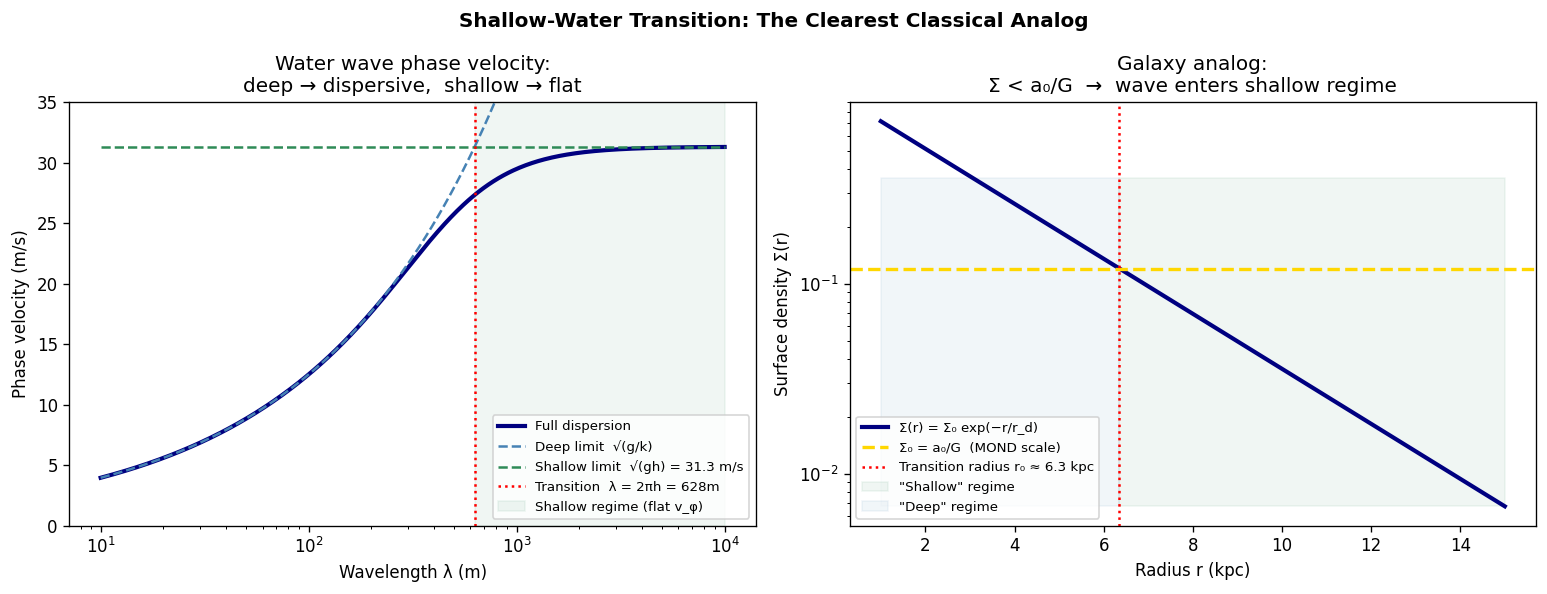
The MOND transition radius r₀ is the galactic analog of the shallow-water
transition wavelength. Below Σ₀ = a₀/G, the density wave changes character:
  Inner disk (Σ > Σ₀):  dispersive Lin-Shu waves, no flat v_φ, no rolling constraint
  Outer disk (Σ < Σ₀):  wave approaches non-dispersive limit, v_φ → flat
  Dark matter = the constraint force required during the transition
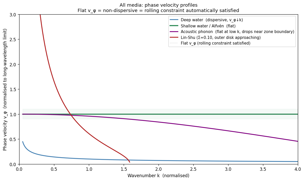
Synthesis: the rolling constraint across media#
Every system in this notebook expresses the same underlying principle:
The rolling constraint is satisfied automatically when the medium is non-dispersive (linear ω∝k). It requires a constraint force (Lagrange multiplier) when the medium is dispersive.
Medium |
Characteristic scale |
Deep/dispersive regime |
Shallow/non-dispersive regime |
Constraint force |
|---|---|---|---|---|
Water waves |
Depth h |
λ << h: v_φ ∝ k^{-1/2} |
λ >> h: v_φ = √(gh) |
Pressure from bottom |
Alfvén waves |
Larmor radius |
ω >> ω_ci: dispersive |
ω << ω_ci: v_φ = v_A |
Magnetic tension |
Acoustic phonon |
Lattice spacing a |
k ~ π/a: dispersive |
k << π/a: v_φ = v_s |
Elastic restoring force |
Galaxy density wave |
Σ₀ = a₀/G |
Σ >> Σ₀: Lin-Shu dispersive |
Σ << Σ₀: approaches v_φ = const? |
Dark matter proxy |
The characteristic scale in each case is where the medium transitions from one regime to the other. The MOND acceleration \(a_0\) is a candidate for the galaxy’s characteristic scale.
What remains open#
Does the Lin-Shu dispersion actually become linear at Σ < Σ₀? The analysis above shows it approaches \(\omega - m\Omega \approx \kappa\) (independent of k), which gives \(v_\phi = \kappa/k\) — not flat. Flatness requires \(k \propto 1/r\), which is the logarithmic spiral condition. The question is whether spiral arms must be logarithmic spirals in this regime (imposed by the dynamics) or whether they can be anything.
Is the evanescent interpretation viable? If the dark matter halo is the exponentially-decaying tail of an evanescent density wave, the profile should be predictable from the wave equation — no free parameters. This is a testable claim.
Rossby-like behavior: do galactic density waves show any phase/group inversion signatures? If so, the angular momentum flux direction would be observationally distinguishable from the particle dark matter prediction.
# Summary figure: all phase velocities on one plot, normalised

k_norm = np.linspace(0.05, 4.0, 500)

# Normalise each to its long-wavelength (k→0) phase velocity
c_shallow = np.sqrt(g * h)

vp_deep_n   = np.sqrt(g / k_norm) / c_shallow          # normalised to shallow limit
vp_shallow_n = np.ones_like(k_norm)                    # = 1 by definition
vp_alfven_n  = np.ones_like(k_norm)                    # always flat
vp_phonon_n  = (2 * np.abs(np.sin(k_norm / 2)) / k_norm)  # normalised phonon

# Lin-Shu: normalised for intermediate Sigma
Sigma_mid = 0.10
rhs_mid   = 1.0 - 2 * np.pi * G * Sigma_mid * k_norm  # kappa normalised to 1
valid_mid = rhs_mid >= 0
vp_linShu_n = np.where(valid_mid, np.sqrt(rhs_mid) / k_norm, np.nan)

fig, ax = plt.subplots(figsize=(10, 6))

ax.plot(k_norm, vp_deep_n,    'steelblue',  lw=2,   label='Deep water  (dispersive, v_φ↓k)')
ax.plot(k_norm, vp_shallow_n, 'seagreen',   lw=2.5, label='Shallow water / Alfvén  (flat)')
ax.plot(k_norm, vp_phonon_n,  'purple',     lw=2,   label='Acoustic phonon  (flat at low k, drops near zone boundary)')
ax.plot(k_norm, vp_linShu_n,  'firebrick',  lw=2,   label='Lin-Shu (Σ=0.10, outer disk approaching)')

ax.axhline(1.0, c='gray', ls=':', lw=1, alpha=0.5, label='Flat v_φ (rolling constraint satisfied)')
ax.fill_between(k_norm, 0.9, 1.1, alpha=0.05, color='seagreen')

ax.set_xlabel('Wavenumber k  (normalised)')
ax.set_ylabel('Phase velocity v_φ  (normalised to long-wavelength limit)')
ax.set_title('All media: phase velocity profiles\n'
             'Flat v_φ = non-dispersive = rolling constraint automatically satisfied',
             fontsize=11)
ax.legend(fontsize=9, loc='upper right')
ax.set_ylim(0, 3)
ax.set_xlim(0, 4)

plt.tight_layout()
plt.show()

print("="*60)
print("SYNTHESIS")
print("="*60)
print("""
The chain:

  MOND scale a₀
      ↓  defines
  Σ₀ = a₀/G  (characteristic surface density)
      ↓  separates
  Inner disk (Σ > Σ₀): dispersive waves,  v_φ = v_φ(k)
  Outer disk (Σ < Σ₀): wave approaches non-dispersive limit
      ↓  requires for flatness
  k ∝ 1/r  (logarithmic spiral arms)
      ↓  produces
  Flat phase velocity v_φ ≈ const
      ↓  satisfies
  Rolling constraint: annulus rolls on wave at constant linear speed
      ↓  via stick-slip locking
  Flat rotation curve ⟨v_circ⟩ ≈ const

Dark matter = Lagrange multiplier of the rolling constraint
            = constraint force that fills the gap between
              what baryonic coupling provides and what rolling requires
            = in wave language: evanescent tail of a mode
              that cannot propagate in the dispersive inner disk
              but decays into the outer disk as an envelope

Open: is the Lin-Shu → flat-v_φ transition provably coincident
with the MOND acceleration threshold?  That would close the chain.
""")
/tmp/ipykernel_2684/2964735423.py:17: RuntimeWarning: invalid value encountered in sqrt
  vp_linShu_n = np.where(valid_mid, np.sqrt(rhs_mid) / k_norm, np.nan)
============================================================
SYNTHESIS
============================================================

The chain:

  MOND scale a₀
      ↓  defines
  Σ₀ = a₀/G  (characteristic surface density)
      ↓  separates
  Inner disk (Σ > Σ₀): dispersive waves,  v_φ = v_φ(k)
  Outer disk (Σ < Σ₀): wave approaches non-dispersive limit
      ↓  requires for flatness
  k ∝ 1/r  (logarithmic spiral arms)
      ↓  produces
  Flat phase velocity v_φ ≈ const
      ↓  satisfies
  Rolling constraint: annulus rolls on wave at constant linear speed
      ↓  via stick-slip locking
  Flat rotation curve ⟨v_circ⟩ ≈ const

Dark matter = Lagrange multiplier of the rolling constraint
            = constraint force that fills the gap between
              what baryonic coupling provides and what rolling requires
            = in wave language: evanescent tail of a mode
              that cannot propagate in the dispersive inner disk
              but decays into the outer disk as an envelope

Open: is the Lin-Shu → flat-v_φ transition provably coincident
with the MOND acceleration threshold?  That would close the chain.