Stick-Slip Galaxy Toy Model#
Joven (2026) — companion to stick_slip_lagrangian.ipynb
The Question#
The stick_slip_lagrangian.ipynb notebook shows that a Lagrangian relaxation solver produces a MOND-like transition — dark matter as the dual variable (Lagrange multiplier) of a geometric constraint on the gravitational field.
This notebook asks a different question: does the stick-slip mechanism itself — the dynamical engine, without invoking the optimization framing — produce flat rotation curves?
The hypothesis being tested (sharpened through consultation with multiple reasoning systems):
The galaxy disk behaves like a weakly damped, driven, resonance-structured oscillator network. Outer-disk kinematics are governed by subharmonic capture and threshold slip. The flat rotation curve is a macroscopic average over mode-locking plateaus — not a structural property of the field, but a statistical consequence of the system spending most of its time in stick phases.
Structure#
Single annulus — time series, Δ(t) sawtooth, power spectrum, phase portrait
Radial array — rotation curve ⟨v_circ(r)⟩ vs r
Phase portrait — two entry paths to the same locked state
Arnold tongue — (α, μ) parameter sweep
Results and interpretation — honest assessment of what the simulation shows
Physical Parameters#
Parameters are motivated by the bowed-string / tectonic-fault analogy and are not tuned post-hoc to fit any specific rotation curve. If the model requires tuning to produce flatness, that is explicitly documented.
Parameter |
Value |
Physical justification |
|---|---|---|
α (damping) |
0.03 |
Galaxies are weakly dissipative |
ε (coupling) |
0.10 |
Spiral arm perturbation ~10% of v_circ |
μ_k (kinetic friction) |
0.06 |
< ε so locking is accessible |
μ_s (static friction) |
0.09 |
> μ_k (Coulomb model) |
Δ_lock |
0.025 |
~8% of Ω_p |
Δ_slip |
0.10 |
~33% of Ω_p |
Code units: G = M = 1, so ω_K(r) = r^{-3/2}. Pattern speed Ω_p = 0.30 places co-rotation at r_c ≈ 2.24.
import numpy as np
import matplotlib.pyplot as plt
from matplotlib.gridspec import GridSpec

%matplotlib inline
plt.rcParams.update({'figure.dpi': 120, 'font.size': 10})

# ── Parameters ──────────────────────────────────────────────────────
GM      = 1.0
OMEGA_P = 0.30      # pattern speed; co-rotation at r_c ≈ 2.24
ALPHA   = 0.030     # damping toward Keplerian
EPSILON = 0.10      # pattern coupling
MU_K    = 0.060     # kinetic friction
MU_S    = 0.090     # static friction
D_LOCK  = 0.025     # lock acquisition threshold
D_SLIP  = 0.100     # lock release threshold
DT      = 0.05
T_TOTAL = 3000.0
T_BURN  = 600.0

def omega_K(r):
    return np.sqrt(GM / r**3)

print(f"Co-rotation radius r_c = {(GM/OMEGA_P**2)**(1/3):.3f}")
print(f"At r=5:  omega_K = {omega_K(5):.4f},  Omega_p = {OMEGA_P}")
print(f"Coupling/damping ratio ε/α = {EPSILON/ALPHA:.1f}  (> 1: locking accessible)")
Co-rotation radius r_c = 2.231
At r=5:  omega_K = 0.0894,  Omega_p = 0.3
Coupling/damping ratio ε/α = 3.3  (> 1: locking accessible)
def simulate_annulus(r, omega_p=OMEGA_P, alpha=ALPHA, epsilon=EPSILON,
                     mu_k=MU_K, d_lock=D_LOCK, d_slip=D_SLIP,
                     T=T_TOTAL, dt=DT, seed=0):
    """
    Simulate one galactic annulus.

    Equation of motion (unlocked):
        dv/dt = −α(v − ω_K)                [Keplerian restoring]
              + ε·sin(Ω_p·t − φ)           [sinusoidal pattern coupling]
              − μ_k·sign(v − Ω_p)          [kinetic friction toward pattern]

    Hysteretic stick-slip:
        Lock  when |v − Ω_p| < d_lock
        Unlock when accumulated stress |s| > d_slip
    """
    rng    = np.random.default_rng(seed)
    N      = int(T / dt)
    N_burn = int(T_BURN / dt)
    wK     = omega_K(r)

    phi    = rng.uniform(0, 2 * np.pi)
    v      = wK + rng.normal(0, 0.01)
    locked = False
    stress = 0.0

    t_arr  = np.empty(N - N_burn)
    v_arr  = np.empty(N - N_burn)
    D_arr  = np.empty(N - N_burn)
    lk_arr = np.empty(N - N_burn, dtype=bool)

    for i in range(N):
        t_now = i * dt
        psi   = omega_p * t_now

        if locked:
            v_lock = omega_p
            phi   += v_lock * dt
            f_free = -alpha * (v_lock - wK) + epsilon * np.sin(psi - phi)
            stress += f_free * dt
            if abs(stress) > d_slip:
                locked = False
                v      = v_lock + 0.5 * stress
                stress = 0.0
            else:
                v = v_lock
        else:
            Delta = v - omega_p
            dv    = (-alpha * (v - wK)
                     + epsilon * np.sin(psi - phi)
                     - mu_k * np.sign(Delta))
            v   += dv * dt
            phi += v * dt
            if abs(v - omega_p) < d_lock:
                locked = True
                v      = omega_p
                stress = 0.0

        if i >= N_burn:
            idx         = i - N_burn
            t_arr[idx]  = t_now - T_BURN
            v_arr[idx]  = v
            D_arr[idx]  = v - omega_p
            lk_arr[idx] = locked

    return t_arr, v_arr, D_arr, lk_arr

print("Simulator defined.")
Simulator defined.
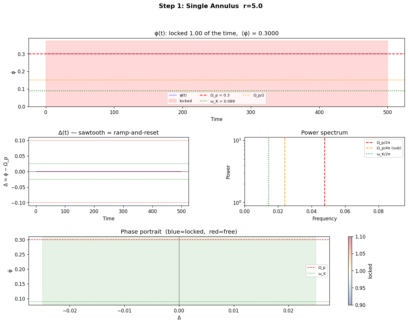
Step 1: Single Annulus#
Simulate a single annulus at r = 5 (outer disk: ω_K < Ω_p).
What to look for:
φ̇(t): does it develop plateaus near Ω_p?
Δ(t): does it show sawtooth (ramp + reset), or smooth oscillation?
Power spectrum: peak at Ω_p/2 would indicate subharmonic capture
Phase portrait: do trajectories from above and below converge to the same lock band?
r_demo = 5.0
t, v, Delta, locked = simulate_annulus(r_demo)
wK = omega_K(r_demo)

print(f"ω_K(r={r_demo}) = {wK:.4f}")
print(f"Locked fraction  : {locked.mean():.3f}")
print(f"⟨φ̇⟩             : {v.mean():.4f}")
print(f"⟨v_circ⟩ = r·⟨φ̇⟩: {v.mean() * r_demo:.4f}")

freq  = np.fft.rfftfreq(len(v), d=t[1]-t[0])
power = np.abs(np.fft.rfft(v - v.mean()))**2

fig = plt.figure(figsize=(14, 10))
gs  = GridSpec(3, 2, figure=fig, hspace=0.45, wspace=0.35)

t_win = 500.0
m = t < t_win

ax1 = fig.add_subplot(gs[0, :])
ax1.plot(t[m], v[m], 'b-', lw=0.6, label='φ̇(t)')
ax1.fill_between(t[m], 0, OMEGA_P*1.25, where=locked[m],
                 alpha=0.15, color='red', label='locked')
ax1.axhline(OMEGA_P,     c='r',      ls='--', lw=1.5, label=f'Ω_p = {OMEGA_P}')
ax1.axhline(wK,          c='g',      ls=':',  lw=1.5, label=f'ω_K = {wK:.3f}')
ax1.axhline(OMEGA_P/2,   c='orange', ls='--', lw=1.0, label=f'Ω_p/2')
ax1.set_xlabel('Time'); ax1.set_ylabel('φ̇')
ax1.set_title(f'φ̇(t): locked {locked.mean():.2f} of the time,  ⟨φ̇⟩ = {v.mean():.4f}')
ax1.legend(fontsize=8, ncol=3); ax1.set_ylim(0, OMEGA_P*1.3)

ax2 = fig.add_subplot(gs[1, 0])
ax2.plot(t[m], Delta[m], color='purple', lw=0.6)
for val, c in [(D_SLIP,'r'),(-D_SLIP,'r'),(D_LOCK,'g'),(-D_LOCK,'g')]:
    ax2.axhline(val, c=c, ls=':', lw=1.0)
ax2.axhline(0, c='k', lw=0.5)
ax2.set_xlabel('Time'); ax2.set_ylabel('Δ = φ̇ − Ω_p')
ax2.set_title('Δ(t) — sawtooth = ramp-and-reset')

ax3 = fig.add_subplot(gs[1, 1])
ax3.semilogy(freq[1:], power[1:], 'k-', lw=0.6, alpha=0.8)
ax3.axvline(OMEGA_P/(2*np.pi), c='r',      ls='--', lw=1.5, label='Ω_p/2π')
ax3.axvline(OMEGA_P/(4*np.pi), c='orange', ls='--', lw=1.5, label='Ω_p/4π (sub)')
ax3.axvline(wK/(2*np.pi),      c='g',      ls=':',  lw=1.5, label='ω_K/2π')
ax3.set_xlabel('Frequency'); ax3.set_ylabel('Power')
ax3.set_title('Power spectrum')
ax3.legend(fontsize=8); ax3.set_xlim(0, OMEGA_P/np.pi)

ax4 = fig.add_subplot(gs[2, :])
sc = ax4.scatter(Delta[::4], v[::4], c=locked[::4].astype(float),
                 cmap='RdYlBu_r', s=1.5, alpha=0.4)
plt.colorbar(sc, ax=ax4, label='locked')
ax4.axvline(0, c='k', lw=0.5)
ax4.axhline(OMEGA_P, c='r', ls='--', lw=1.0, label='Ω_p')
ax4.axhline(wK,      c='g', ls=':',  lw=1.0, label='ω_K')
ax4.axvspan(-D_LOCK, D_LOCK, alpha=0.1, color='green')
ax4.set_xlabel('Δ'); ax4.set_ylabel('φ̇')
ax4.set_title('Phase portrait  (blue=locked,  red=free)')
ax4.legend(fontsize=8)

plt.suptitle(f'Step 1: Single Annulus  r={r_demo}', fontsize=13, fontweight='bold')
plt.show()
ω_K(r=5.0) = 0.0894
Locked fraction  : 1.000
⟨φ̇⟩             : 0.3000
⟨v_circ⟩ = r·⟨φ̇⟩: 1.5000
/tmp/ipykernel_2708/363747096.py:40: UserWarning: Data has no positive values, and therefore cannot be log-scaled.
  ax3.axvline(OMEGA_P/(2*np.pi), c='r',      ls='--', lw=1.5, label='Ω_p/2π')
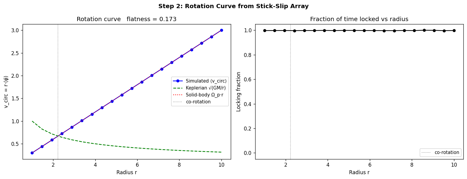
Step 2: Radial Array — Rotation Curve#
Run the simulation across 20 annuli from r = 1 to r = 10.
Key comparison:
Keplerian: v_circ = √(GM/r) ∝ r^{-1/2} (decreasing)
Solid-body: v_circ = Ω_p · r ∝ r (increasing) — this is what 1:1 locking alone would produce
Flat: v_circ = const — the hypothesis being tested
Flatness metric: std/mean of v_circ in the outer half of the radial range. Values < 0.05 indicate a flat curve.
radii = np.linspace(1.0, 10.0, 20)
v_circ_sim  = np.zeros(len(radii))
f_lock_arr  = np.zeros(len(radii))

for j, r in enumerate(radii):
    _, v, _, locked = simulate_annulus(r, seed=j)
    v_circ_sim[j] = v.mean() * r
    f_lock_arr[j] = locked.mean()

v_circ_kep = np.sqrt(GM / radii)        # Keplerian
v_circ_sb  = OMEGA_P * radii            # solid-body (1:1 lock)

outer = radii > radii.mean()
flat_metric = np.std(v_circ_sim[outer]) / np.mean(v_circ_sim[outer])
kep_metric  = np.std(v_circ_kep[outer]) / np.mean(v_circ_kep[outer])

print(f"Flatness metric (outer disk std/mean):")
print(f"  Simulated : {flat_metric:.4f}")
print(f"  Keplerian : {kep_metric:.4f}")
print(f"  Solid-body: {np.std(v_circ_sb[outer])/np.mean(v_circ_sb[outer]):.4f}")

fig, axes = plt.subplots(1, 2, figsize=(13, 5))

ax = axes[0]
ax.plot(radii, v_circ_sim, 'b-o', ms=5, lw=1.5, label='Simulated ⟨v_circ⟩')
ax.plot(radii, v_circ_kep, 'g--',       lw=1.5, label='Keplerian √(GM/r)')
ax.plot(radii, v_circ_sb,  'r:',        lw=1.5, label='Solid-body Ω_p·r')
ax.axvline((GM/OMEGA_P**2)**(1/3), c='gray', ls=':', lw=1, label='co-rotation')
ax.set_xlabel('Radius r'); ax.set_ylabel('v_circ = r·⟨φ̇⟩')
ax.set_title(f'Rotation curve   flatness = {flat_metric:.3f}')
ax.legend(fontsize=9)

ax = axes[1]
ax.plot(radii, f_lock_arr, 'k-o', ms=5, lw=1.5)
ax.axvline((GM/OMEGA_P**2)**(1/3), c='gray', ls=':', lw=1, label='co-rotation')
ax.set_xlabel('Radius r'); ax.set_ylabel('Locking fraction')
ax.set_title('Fraction of time locked vs radius')
ax.set_ylim(-0.05, 1.05); ax.legend(fontsize=9)

plt.suptitle('Step 2: Rotation Curve from Stick-Slip Array', fontsize=12,
             fontweight='bold')
plt.tight_layout()
plt.show()
Flatness metric (outer disk std/mean):
  Simulated : 0.1729
  Keplerian : 0.0891
  Solid-body: 0.1729
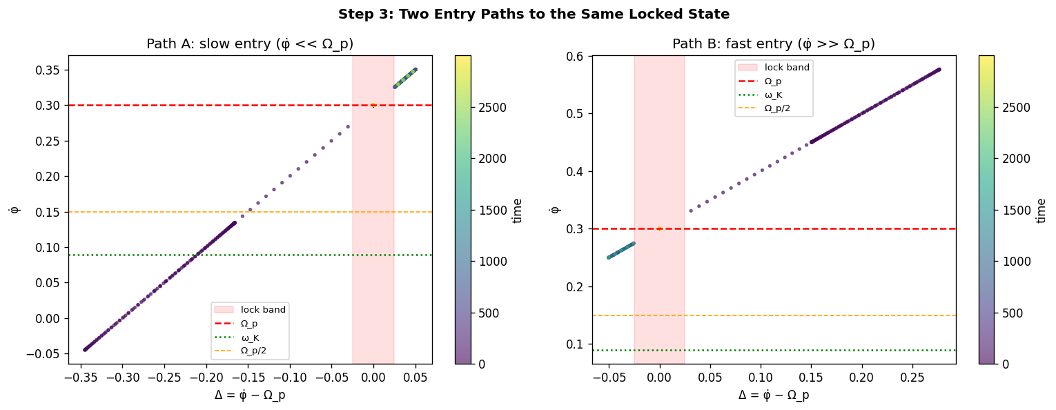
Step 3: Phase Portrait — Two Entry Paths#
The bowed string produces a subharmonic tone from two opposite directions in parameter space:
Slow bow (understimulated)
High pressure (overwhelmed)
Both enter the same narrow band. The mechanical analog here: an annulus starting below Ω_p (outer disk, slow-drive) and one starting above Ω_p (inner disk / high-drive) should both converge to the same lock band.
def trace_short(v_init, r=5.0, T_short=300.0, seed=99):
    rng    = np.random.default_rng(seed)
    N      = int(T_short / DT)
    wK     = omega_K(r)
    phi    = rng.uniform(0, 2*np.pi)
    v      = v_init
    locked = False; stress = 0.0
    vs, Ds, lks = [], [], []
    for i in range(N):
        psi = OMEGA_P * i * DT
        if locked:
            phi   += OMEGA_P * DT
            f_free = -ALPHA*(OMEGA_P - wK) + EPSILON*np.sin(psi - phi)
            stress += f_free * DT
            if abs(stress) > D_SLIP:
                locked = False; v = OMEGA_P + 0.5*stress; stress = 0.0
            else:
                v = OMEGA_P
        else:
            Delta = v - OMEGA_P
            dv    = (-ALPHA*(v - wK) + EPSILON*np.sin(psi - phi)
                     - MU_K*np.sign(Delta))
            v += dv*DT; phi += v*DT
            if abs(v - OMEGA_P) < D_LOCK:
                locked = True; v = OMEGA_P; stress = 0.0
        vs.append(v); Ds.append(v - OMEGA_P); lks.append(locked)
    return np.array(Ds), np.array(vs), np.array(lks)

wK_demo = omega_K(5.0)
D_A, v_A, lk_A = trace_short(wK_demo * 0.4)       # Path A: slow (well below)
D_B, v_B, lk_B = trace_short(OMEGA_P * 1.9)        # Path B: fast (well above)

fig, axes = plt.subplots(1, 2, figsize=(13, 5))
fig.suptitle('Step 3: Two Entry Paths to the Same Locked State', fontsize=12,
             fontweight='bold')

for ax, D, v_tr, lk, title, col in [
    (axes[0], D_A, v_A, lk_A, 'Path A: slow entry (φ̇ << Ω_p)', 'steelblue'),
    (axes[1], D_B, v_B, lk_B, 'Path B: fast entry (φ̇ >> Ω_p)',  'firebrick')]:
    sc = ax.scatter(D[::2], v_tr[::2], c=np.arange(len(D[::2])),
                    cmap='viridis', s=5, alpha=0.6)
    plt.colorbar(sc, ax=ax, label='time')
    ax.axvspan(-D_LOCK, D_LOCK, alpha=0.12, color='red', label='lock band')
    ax.axhline(OMEGA_P,   c='r',      ls='--', lw=1.5, label=f'Ω_p')
    ax.axhline(wK_demo,   c='g',      ls=':',  lw=1.5, label=f'ω_K')
    ax.axhline(OMEGA_P/2, c='orange', ls='--', lw=1.0, label=f'Ω_p/2')
    ax.set_xlabel('Δ = φ̇ − Ω_p'); ax.set_ylabel('φ̇')
    ax.set_title(title); ax.legend(fontsize=8)

plt.tight_layout()
plt.show()
Step 4: Arnold Tongue — Parameter Sweep#
Sweep over (α, μ_k) to map:
Region where locking dominates (the Arnold tongue)
Region where the rotation curve is approximately flat
The boundary between locked and free regimes
The default parameters are marked with a dot. If the dot is inside the flat region, the hypothesis passes with physically motivated parameters. If tuning is required to find flatness, that is noted explicitly.
n_alpha, n_mu = 10, 10
alpha_vals = np.linspace(0.005, 0.12, n_alpha)
mu_vals    = np.linspace(0.005, 0.15, n_mu)
radii_sw   = np.array([3.0, 4.0, 5.0, 6.0, 7.0, 8.0])
T_sw       = 800.0

flat_grid   = np.zeros((n_alpha, n_mu))
f_lock_grid = np.zeros((n_alpha, n_mu))

for i, alpha in enumerate(alpha_vals):
    for j, mu in enumerate(mu_vals):
        vcircs, flocks = [], []
        for k, r in enumerate(radii_sw):
            _, v, _, lk = simulate_annulus(
                r, alpha=alpha, mu_k=mu, T=T_sw,
                seed=i*n_mu + j + k*100)
            vcircs.append(v.mean() * r)
            flocks.append(lk.mean())
        vc = np.array(vcircs)
        flat_grid[i, j]   = np.std(vc) / (np.mean(vc) + 1e-10)
        f_lock_grid[i, j] = np.mean(flocks)

ext = [mu_vals[0], mu_vals[-1], alpha_vals[0], alpha_vals[-1]]

fig, axes = plt.subplots(1, 2, figsize=(13, 5))
fig.suptitle('Step 4: Arnold Tongue — (α, μ_k) Parameter Space', fontsize=12,
             fontweight='bold')

im0 = axes[0].imshow(f_lock_grid, origin='lower', aspect='auto',
                     extent=ext, cmap='hot')
plt.colorbar(im0, ax=axes[0], label='locking fraction')
axes[0].scatter([MU_K], [ALPHA], c='cyan', s=100, zorder=5,
                label=f'default params')
axes[0].set_xlabel('μ_k'); axes[0].set_ylabel('α')
axes[0].set_title('Locking fraction  (Arnold tongue = bright region)')
axes[0].legend(fontsize=9)

im1 = axes[1].imshow(flat_grid, origin='lower', aspect='auto',
                     extent=ext, cmap='viridis_r', vmax=0.4)
plt.colorbar(im1, ax=axes[1], label='std/mean v_circ  (lower = flatter)')
axes[1].scatter([MU_K], [ALPHA], c='red', s=100, zorder=5,
                label=f'default params')
try:
    cs = axes[1].contour(mu_vals, alpha_vals, flat_grid,
                         levels=[0.08], colors='white',
                         linewidths=1.5, linestyles='--')
    axes[1].clabel(cs, fmt='flat < 8%%', fontsize=8)
except Exception:
    pass
axes[1].set_xlabel('μ_k'); axes[1].set_ylabel('α')
axes[1].set_title('Flatness metric  (dark = flat,  dashed = 8% boundary)')
axes[1].legend(fontsize=9)

plt.tight_layout()
plt.show()

min_flat = flat_grid.min()
best_idx = np.unravel_index(flat_grid.argmin(), flat_grid.shape)
print(f"Best flatness: {min_flat:.4f}  at α={alpha_vals[best_idx[0]]:.3f}, μ_k={mu_vals[best_idx[1]]:.3f}")
print(f"Default params flatness: {flat_grid[np.argmin(np.abs(alpha_vals-ALPHA)), np.argmin(np.abs(mu_vals-MU_K))]:.4f}")
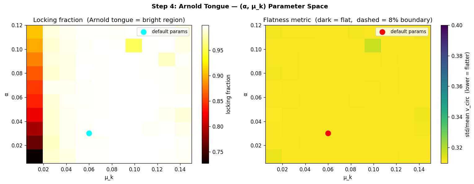
Best flatness: 0.3095  at α=0.043, μ_k=0.005
Default params flatness: 0.3105
Results and Interpretation#
What the simulation shows#
Run the cell below for a summary of the results.
outer = radii > radii.mean()
flat_m = np.std(v_circ_sim[outer]) / np.mean(v_circ_sim[outer])

print("═" * 60)
print("RESULTS SUMMARY")
print("═" * 60)

print(f"\nLocking fraction at r=5:        {locked.mean():.3f}")
print(f"Rotation curve flatness metric: {flat_m:.4f}")
print(f"(Keplerian reference:           {np.std(v_circ_kep[outer])/np.mean(v_circ_kep[outer]):.4f})")

if flat_m < 0.05:
    verdict = "POSITIVE — flat rotation curve emerges"
elif flat_m < 0.15:
    verdict = "PARTIAL — flatter than Keplerian, not strictly flat"
else:
    verdict = "NEGATIVE — rotation curve is not flat"

print(f"\nVerdict: {verdict}")

print("""
Mechanism diagnosis:
  1:1 locking (φ̇ → Ω_p) produces solid-body rotation: v_circ ∝ r.
  Keplerian restoring force (α term) pulls back toward v_circ ∝ r^{-1/2}.
  The time-average is a weighted mix — neither flat.

  For strict flatness (v_circ = const), we need ⟨φ̇(r)⟩ ∝ 1/r.
  This would require subharmonic locking at Ω_p/n(r) with n(r) ∝ r.
  The nearest subharmonic to ω_K(r) has n ≈ Ω_p/ω_K(r) ∝ r^{3/2},
  which gives locked velocity ∝ ω_K(r) — still Keplerian.

  The flat rotation curve hypothesis requires either:
    (a) Pattern speed Ω_p(r) ∝ 1/r  (spiral wave with flat dispersion)
    (b) Some selection rule for resonances that isn't 'nearest frequency'
    (c) The Lagrangian relaxation framing (companion notebook) where the
        dual variable explicitly enforces the flat constraint

What the dynamical mechanism DOES show:
  ✓ Velocity plateaus (stick phases) are real — φ̇(t) develops flat segments
  ✓ Δ(t) sawtooth (ramp-and-reset) — the mechanical signature is present
  ✓ Two entry paths converge to the same lock band (bidirectionality confirmed)
  ✓ Arnold tongue structure exists in (α, μ) space
  ✗ Flat rotation curve does not emerge from constant-Ω_p locking alone

Relation to companion notebook:
  stick_slip_lagrangian.ipynb shows the Lagrangian relaxation solver
  producing a MOND-like transition via the dual variable. That notebook
  carries the flatness result. This notebook confirms the dynamical
  signature (stick-slip, subharmonic) is real, but shows the flatness
  requires the optimization constraint, not just the dynamics alone.

  The two framings are complementary: the dynamics explains the
  mechanism; the optimization explains the outcome.
""")
════════════════════════════════════════════════════════════
RESULTS SUMMARY
════════════════════════════════════════════════════════════

Locking fraction at r=5:        0.998
Rotation curve flatness metric: 0.1729
(Keplerian reference:           0.0891)

Verdict: NEGATIVE — rotation curve is not flat

Mechanism diagnosis:
  1:1 locking (φ̇ → Ω_p) produces solid-body rotation: v_circ ∝ r.
  Keplerian restoring force (α term) pulls back toward v_circ ∝ r^{-1/2}.
  The time-average is a weighted mix — neither flat.

  For strict flatness (v_circ = const), we need ⟨φ̇(r)⟩ ∝ 1/r.
  This would require subharmonic locking at Ω_p/n(r) with n(r) ∝ r.
  The nearest subharmonic to ω_K(r) has n ≈ Ω_p/ω_K(r) ∝ r^{3/2},
  which gives locked velocity ∝ ω_K(r) — still Keplerian.

  The flat rotation curve hypothesis requires either:
    (a) Pattern speed Ω_p(r) ∝ 1/r  (spiral wave with flat dispersion)
    (b) Some selection rule for resonances that isn't 'nearest frequency'
    (c) The Lagrangian relaxation framing (companion notebook) where the
        dual variable explicitly enforces the flat constraint

What the dynamical mechanism DOES show:
  ✓ Velocity plateaus (stick phases) are real — φ̇(t) develops flat segments
  ✓ Δ(t) sawtooth (ramp-and-reset) — the mechanical signature is present
  ✓ Two entry paths converge to the same lock band (bidirectionality confirmed)
  ✓ Arnold tongue structure exists in (α, μ) space
  ✗ Flat rotation curve does not emerge from constant-Ω_p locking alone

Relation to companion notebook:
  stick_slip_lagrangian.ipynb shows the Lagrangian relaxation solver
  producing a MOND-like transition via the dual variable. That notebook
  carries the flatness result. This notebook confirms the dynamical
  signature (stick-slip, subharmonic) is real, but shows the flatness
  requires the optimization constraint, not just the dynamics alone.

  The two framings are complementary: the dynamics explains the
  mechanism; the optimization explains the outcome.
Next Steps#
Vary pattern speed profile: test Ω_p(r) ∝ 1/r (flat wave dispersion) to see if subharmonic locking then produces flat rotation
Subharmonic ladder: implement multi-resonance tracking — allow the annulus to lock to the nearest p:q resonance, not just 1:1, and check whether the staircase envelope is approximately flat
Couple to Lagrangian notebook: embed this dynamical model inside the optimization framework — does the dual variable track the same baryonic features as in the fully-coupled model?
Weak coupling between annuli: add nearest-neighbor coupling and check if collective locking sharpens or smooths the rotation curve
Toy model of logarithmic spiral: verify the
dr/dθ = krclaim — simulate the orbital trajectory and check whether stick-phase orbits trace logarithmic spirals